Formal Languages and Automata
Zhengfeng Ji
Lecture 1: Formal Languages and Automata
About This Course
Welcome
This is an incomplete set of notes prepared by Zhengfeng Ji for the course. Please do not distribute.
Formal languages and automata
Lecturer
Zhengfeng Ji
Office: 1-707, Ziqiang Technology Building
Email: jizhengfeng@tsinghua.edu.cn
Research direction: quantum computing, theory of computing.
Teaching assistants
Huiping Lin (lhp22@mails.tsinghua.edu.cn)
Aochu Dai (dac22@mails.tsinghua.edu.cn)
Shenghan Gao (sh-gao24@mails.tsinghua.edu.cn)
Third time I teach this course in Tsinghua
Your feedback is welcome
Computation and mathematics
Also known as Introduction to the ToC in some universities
Key observation
Computation, Mathematics, Logic
Computational problems, devices, and processes can be viewed as mathematical objects.
One interesting connection between computation and mathematics, which is particularly important from the viewpoint of this course, is that mathematical proofs and computations performed by the models we will discuss throughout this course have a low-level similarity: they both involve symbolic manipulations according to fixed sets of rules. (Watrous lecture notes)
We will study different types of recursions, Kleene star, context-free grammars, and Turing machines.
What you will learn in this subject
- Finite automata and regular expressions
- Pushdown automata and context-free grammars (CFG)
- Turing machine and computability, basic complexity theory
More importantly, we hope that you will learn how to write definitions/proofs rigorously;
Improve mathematical maturity.
I offer a follow-up course next semester called Introduction to Theoretical Computer Science, which covers lambda calculus, advanced computability, complexity theory, probabilistic computation, cryptography, and propositions as types.
See lecture notes at http://itcs.finite-dimensional.space
Teaching and learning
We use chalk and board.
The chalk and board way is better for teaching and learning theoretical subjects.
In How to speak from Patrick Winston (MIT), it is argued that chalk/board is the right tool for speaking when the purpose is informing.
Please be actively involved!
Reviewing after each class is highly recommended.
We will hand out notes after each class for you to review the materials covered in class.
The subject could be challenging for many of you.
It has a different style and different set of requirements.
Pause and think about the problem or theorem by yourself before you see the proof.
Barak: Even a five-minute attempt to solve the problem by yourself will significantly improve your understanding of the topic.
Textbook
Introduction to Automata Theory, Languages, and Computation (3rd ed), by John Hopcroft, Rajeev Motwani, Jeffrey Ullman.
Hopcroft: In 1986, he received the Turing Award (jointly with Robert Tarjan) for fundamental achievements in the design and analysis of algorithms and data structures. He helped to build research centers in Shanghai Jiaotong and Peking U.
Motwani: Gödel Prize for PCP theorem. Author of another excellent textbook Randomized Algorithms. Youngest of the three. But unfortunately, he passed away in 2009.
Ullman: Turing award (2020) for his work on compilers. Author of the Dragon book Compilers: principles, techniques, & tools. He was the Ph.D. advisor of Sergey Brin, one of the co-founders of Google.
- Other materials:
- Introduction to the Theory of Computation, Michael Sipser
- Watrous lecture notes (https://cs.uwaterloo.ca/~watrous/ToC-notes/)
- Lecture notes: http://fla.finite-dimensional.space
Homework
About 12 assignments
Highly recommended to complete them on time
Grading
Mid-term: 20%
Attendance & homework: 10%
Final exam: 70%
Q & A
Online: Wechat group, learn.tsinghua.edu.cn, email
Office hour: 4-5 pm Tuesday
Why Learning This Subject
Ancient materials (mostly developed between 30's and 60's)
Finite automata
Simple examples of finite automata
Simple model enables deep understanding of its properties and efficient algorithms for manipulating it.
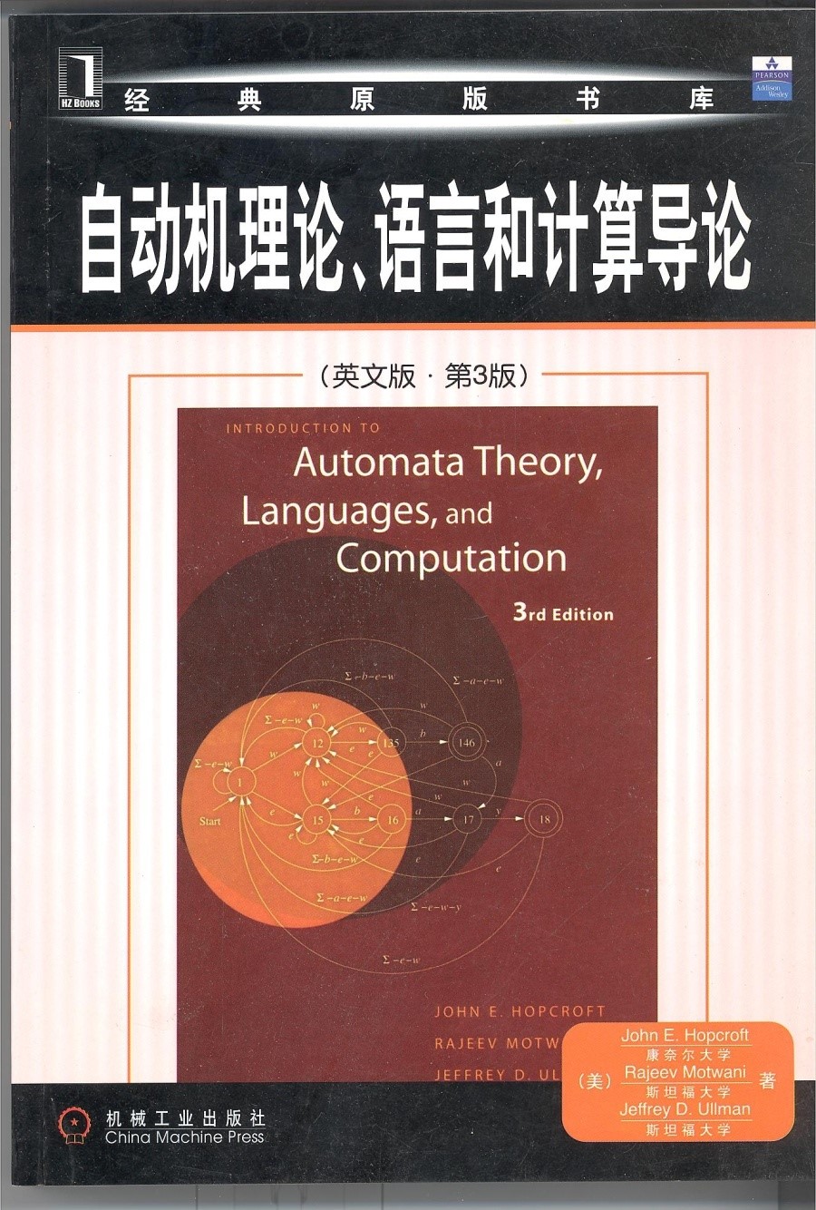
Example 1. Figure 1.1, push a button and switch between on and off, starting from off.
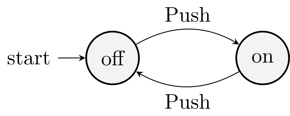
Example 2. Search for the word the
Finite automata are a valuable model for many important kinds of hardware and software.
- Specification, verification, and model checking of systems of finite states, circuits, and communication protocols
- Lexical analyzer for compilers
- Text search
When and how is it discovered
[McCulloch and Pitts, A logical calculus of ideas immanent in nervous activity, 1943]
[Kleene, Representation of events in nerve nets and finite automata, 1956]
[Rabin and Scott, Finite automata and their decision problems, 1959]
Regular expression
\([A-Z][a-z]*\) matches Computer
Context-free grammars
Grammars are useful models when designing software that processes data with a recursive structure.
Program languages
Compilers never enter a dead loop.
Pushdown automata
Machine with a single stack.
Turing machine
What can a computer do at all?
Hilbert 1928 Entscheidungsproblem (cf. Hilbert 10th problem about Diophantine equations)
The problem asks for an algorithm that considers, as input, a statement and answers Yes or No according to whether the statement is valid.
What cannot be done on a computer?
We must know. We will know.
The epitaph on his tombstone in Göttingen consists of the famous lines he spoke after his retirement address to the Society of German Scientists and Physicians on 8 September 1930.
What is computation?
Church: Lambda calculus (\(\lambda x . x^2 + 2\))
Gödel: Recursive functions
Turing: Turing machines (age 24)
You: C, Python, Java, …
TM is intuitive capture of computation, and Gödel is convinced.
It's like waiting for the bus. We waited for 2000 years for a formal definition of computation; three buses come along at the same time.
All equivalent: Is mathematics invented or discovered?
Church-Turing thesis
Logic and computation
Gödel's incompleteness: The first incompleteness theorem states that no consistent system of axioms whose theorems can be listed by an effective procedure (i.e., an algorithm) is capable of proving all truths about the arithmetic of natural numbers.
What can a computer do efficiently?
Space/time-bounded TMs
Extended Church-Turing thesis
Basics of FL&A
Sets and countability
The naive set theory treats the concept of a set to be self-evident. This will not be problematic for this course, but it does lead to problems and paradoxes—such as Russell's paradox—when it is pushed to its limits.
Bertrand Russell Russell's paradox. Let S be the set of all sets that are not elements of themselves: \(S = \{T : T \text{ is not in } T\}\). Is it the case that \(S\) is an element of itself? (Self-reference)
The size of a finite set \(S\) is denoted \(\abs{S}\).
Sets can also be infinite.
Definition. A set \(A\) is countable if either (i) \(A\) is empty, or (ii) there exists an onto (or surjective) function of the form \(f : \mathbb{N} \rightarrow A\). If a set is not countable, we say it is uncountable.
Power sets:
\(2^A\) or \(P(A)\)
More generally: What is \(A^B\)?
Theorem. The set \(\mathbb{Q}\) of rational numbers is countable.
Theorem (Cantor). The power set of the natural numbers, \(P(\mathbb{N})\), is uncountable.
There is a technique at work in this proof known as diagonalization. It is a fundamentally important technique in the theory of computation, and we will see instances of it later.
Central concepts of formal languages
Alphabets
An alphabet is a finite nonempty set of symbols.
\(\Sigma = \{0,1\}\)
\(\Sigma = \{a, b, c, \ldots, z\}\)
Strings
Strings are sequences of symbols chosen from an alphabet.
0101 is a seq from the alphabet \(\{0,1\}\)
Empty string: \(\eps\)
The length of string \(\abs{010} = 3\)
powers of an alphabet
\(\Sigma^3\)
The set of all strings over an alphabet \(\Sigma^*\)
\(\Sigma^* = \cup_{n\ge 0} \Sigma^n\)
\(\Sigma^+\)
Concatenation \(xy\)
Language
Subset \(L\) of \(\Sigma^*\)
Set formers as a way to define languages
The set of binary numbers whose value is a prime
Problems
In automata theory, a problem is the question of deciding whether a given string is a member of some particular language.
Union/concatenation/closure (star, Kleene closure)
\(L \cup R\)
\(LR\)
\(L^* = \bigcup_{i=0}^\infty L^i\)
Proof techniques
Proofs about sets
Ex. \(R \cup (S \cap T) = (R \cup S) \cap (R \cup T)\)
Proofs by contradiction
Proofs by inductions
Inductive proofs
Prove a statement about \(S(n)\) for integer \(n \ge n_0\)
Basis: \(S(n_0)\) is true
Induction: if \(S(n)\) then \(S(n+1)\) for \(n \ge n_0\)
Mutual inductions
Prove statements together!
Example. In the on-off automata,
\(S_1(n)\): the automata is in the state off after \(n\) if only if \(n\) is even.
\(S_2(n)\): the automata is in the state on after \(n\) if only if \(n\) is odd.
Structural inductions
The most important proof technique for automata theory and programming languages
Ex. Trees
Basis: A single node is a tree, and that node is the root of the tree.
Induction: If \(T_1, T_2, \ldots, T_k\) are trees, then we can form a new tree as follows:
- Begin with a new node \(N\), which is the root of the new tree.
- Add copies of all the trees \(T_1, \ldots, T_k\)
- Add edges from node \(N\) to the roots of each of the trees \(T_1, \ldots, T_k\)
Theorem. Every tree has one more node than it has edges.
Proof. Use structral induction. Basis. The tree has a single node. Induction. Assume the claim is true for \(T_1, \ldots, T_k\), …
Ex. Expression
Basis: Any number or letter is an expression.
Induction: If \(E\) and \(F\) are expressions, then so are \(E + F\), \(E * F\), and \((E)\).
Reading
Lecture 2: Finite Automata
Outline
DFA, NFA, and \(\eps\)-NFA
An Informal Picture
Read Sec 2.1 of the textbook.
External actions drive the changes in the internal state.
What is a Finite Automata
Examples
Finite automata are very simple models of computation that will be our focus for the next four to five weeks.
Computation with finite memory
Example 1. A finite automaton for the light switch.
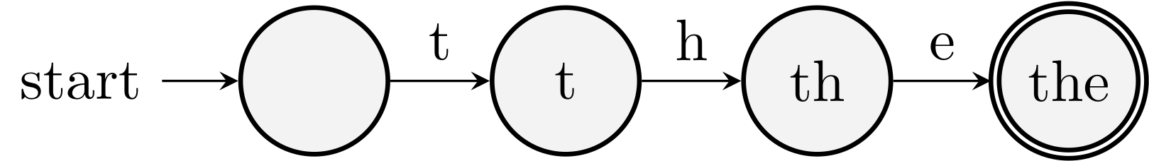
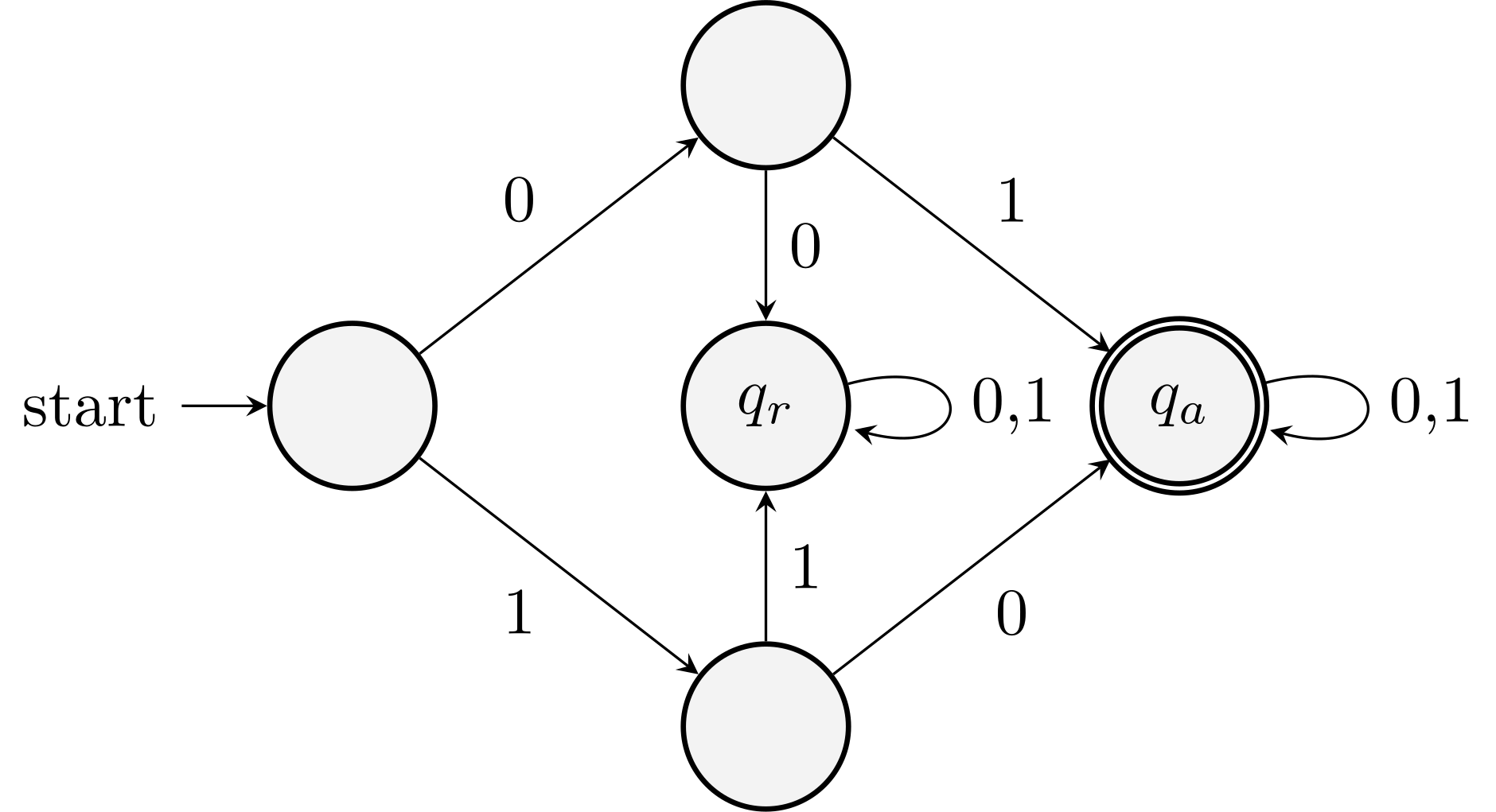
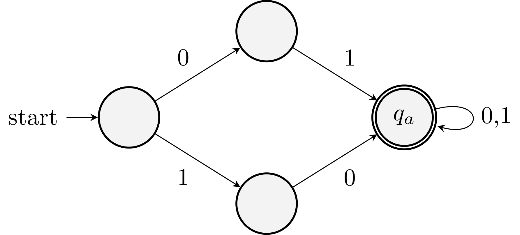
Example 2. A finite automaton for accepting all binary strings that has length at least two and the first two letters are different.
Example 3. A finite automaton for accepting all binary strings that are \(4 \pmod{7}\).
0 1 \(\rightarrow\) 0 0 1 1 2 3 2 4 5 3 6 0 \(*\) 4 1 2 5 3 4 6 5 6 We will talk about deterministic finite automata first.
Models we will not cover:
Mealy machines (outputs determined by the input symbol and current state)
Moore machines (outputs determined by the current state only)
Formal definition of DFA
Mathematical definition
- A finite set of states \(Q\)
- Input alphabet: A finite set of symbols \(\Sigma\)
- Transition function \(\delta : Q \times \Sigma \rightarrow Q\)
- A start state \(q_0 \in Q\)
- A set of final states \(F \subseteq Q\)
A deterministic finite automaton (DFA) is a five-tuple \(A = (Q, \Sigma, \delta, q_0, F)\)
Transition diagrams
See Examples 1 and 2.
They are best for visualization
Transition tables
Columns of state transitions
See Example 3 above.
They are machine friendly
How a DFA processes strings
It starts in the start state.
It enters a new state according to the transition function \(\delta\).
It accepts if and only if the final state is accepting.
Examples
Example. Design a DFA that accepts all and only the strings of 0's and 1's that have a \(01\) somewhere. That is, \(L = \{w \mid w = x01y \}\).
The automaton needs to remember:
- Has it seen a \(01\)? If so, accepts regardless of further input.
- Has it never seen a \(01\) but the most recent input is \(0\)?
- Has it never seen a \(0\)?
This gives us a simple automaton with three states.
Example. Design a DFA that accepts all and only the strings of 0's and 1's that have \(01\) as the last two letters. That is, \(L = \{w \mid w = x01 \}\).
Note the differences at the accepting node.
Example. Design a DFA that accepts all strings over \(\{0,1\}\) in which there are odd number of occurrences of 01.
For example, \(01000\) should be accepted while \(01001\) should not.

The language of a DFA
What do we mean by calling a language regular?
A language is regular if it is the set of strings accepted by a finite automata.
Regular: arranged in or constituting a constant or definite pattern, especially with the same space between individual instances.
Succinct and precise, and leaves no ambiguities
Extended transition function
How to define \(\hat{\delta}(q, w)\) for a string \(w\)?
Write \(w = xa\) and inductively define \(\hat{\delta}\).
We can write the language of the DFA using extended transition function: \(L(A) = \bigl\{w \mid \hat{\delta}(q_0, w) \in F\bigr\}\).
Are regular languages countable or not?
Yes!
This means that there are languages \(L \subseteq {\{0,1\}}^*\) that are not regular.
Nondeterministic Finite Automata
Nondeterminism
The machine can make guesses (non-deterministic choices) during computation.
Example
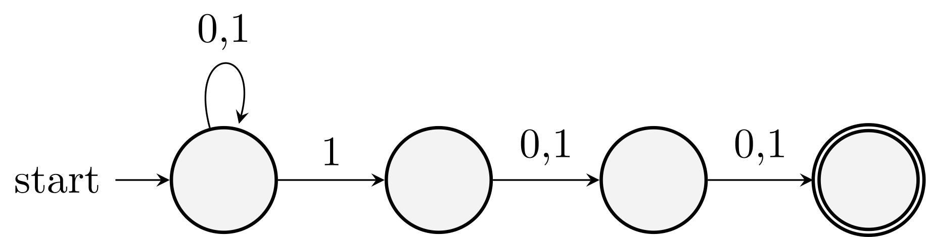
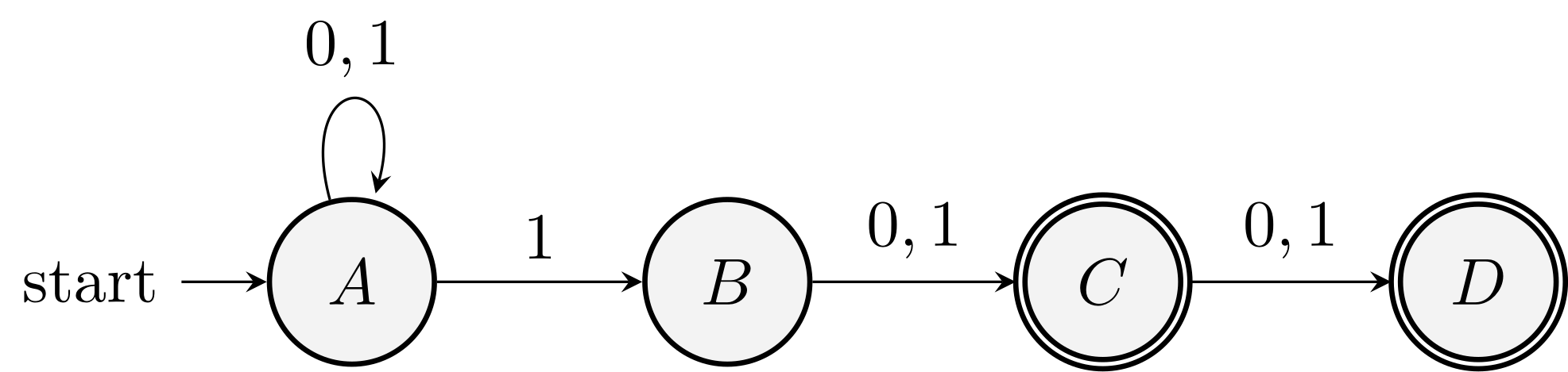
Binary strings whose 3rd letter from the end is a \(1\).
Example 2 with NFA:
Dead states and DFAs missing some transitions
They are not DFAs by definition, but they are in fact NFAs.
See Example 2.
Formal definition
It is still a five-tuple, but now the transition function is different. (The only difference)
Nondeterminism is reflected in the fact that \(\delta(q, a)\) is a set of states representing all possible target states when the current state is \(q\), and the input symbol is \(a\).
Extended transition function
- Write \(w=xa\) and take the union of \(\delta(p_i, a)\) for all \(p_i \in \hat{\delta}(p_0, x)\).
The language of an NFA
Intuition and formal definition: \[\begin{equation*} L(A) = \bigl\{w \mid \hat{\delta}(q_0, w) \cap F \ne \emptyset \bigr\}. \end{equation*}\]
The string is in the languages as long as there exists a nondeterministic choice of path leading to acceptance.
DFA and NFA Equivalence
What does it mean?
Any language \(L\) has a DFA if and only if it has an NFA.
The direction from DFA to NFA is easy as any DFA is a special NFA.
NFA to DFA: idea
Subset Construction
The transition in NFA is to a set of states (representing the nondeterministic choices).
Can we use a set of states (of the NFA) as the state of a DFA?
Transition: Union of target states for each state in the set.
NFA to DFA: proof
Let \(N\) be an NFA. We design a DFA \(D\) such that \(L(D) = L(N)\).
The five components of \(D\) are:
The set of states \(Q_D\) is the power set \(2^{Q_N}\).
The alphabet is the same \(\Sigma\).
The transition rule \(\delta_D\) is
\[\begin{equation*} \delta_D(S, a) = \bigcup_{q\in S} \delta_N(q, a). \end{equation*}\]
Start state \(\{q_0\}\).
Final states: any set that has nontrivial overlap with \(F\).
Now we need to show that the construction works, that is, \(w \in L(N)\) if and only if \(w \in L(D)\).
\(w \in L(N)\) means \(\delta_N(q_0, w)\) contains states in \(F\) and \(w \in L(D)\) means \(\delta_D(\{q_0\}, w)\) contains states in \(F\).
Induction on the length \(\abs{w}\) and prove that \(\delta_N(q_0, w) = \delta_D(\{q_0\}, w)\).
See Theorem 2.11 of the textbook.
Comments
DFA simulation of NFA could have exponentially large number of states.
Example: all bit strings whose \(n\)-th symbol from the end is \(1\).
Show that any DFA accepting those strings will have at least \(2^n\) states. (Pigeonhole principle)
Yet there is a NFA with \(n+1\) states for this. (The NFA first loops for a while on \(0,1\) and then move \(n\) steps sequentially).
Lecture 3: Regular Expressions and Languages
Finite Automata With Epsilon-Transitions
It is an NFA allowed to make a transition spontaneously without receiving an input symbol.
Why?
It has the same power as DFAs and NFAs.
But they are sometimes easier to use and construct, for example, when we discuss regular expressions.
An example
Consider Example 2.18 of the textbook.
\(\eps\) \({+}, {-}\) \(.\) \(0,1,\ldots,9\) \(\rightarrow q_0\) \(\{q_1\}\) \(\{q_1\}\) \(\emptyset\) \(\emptyset\) \(q_1\) \(\emptyset\) \(\emptyset\) \(\{q_2\}\) \(\{q_1, q_4\}\) \(q_2\) \(\emptyset\) \(\emptyset\) \(\emptyset\) \(\{q_3\}\) \(q_3\) \(\{q_5\}\) \(\emptyset\) \(\emptyset\) \(\{q_3\}\) \(q_4\) \(\emptyset\) \(\emptyset\) \(\{q_3\}\) \(\emptyset\) \(*q_5\) \(\emptyset\) \(\emptyset\) \(\emptyset\) \(\emptyset\) 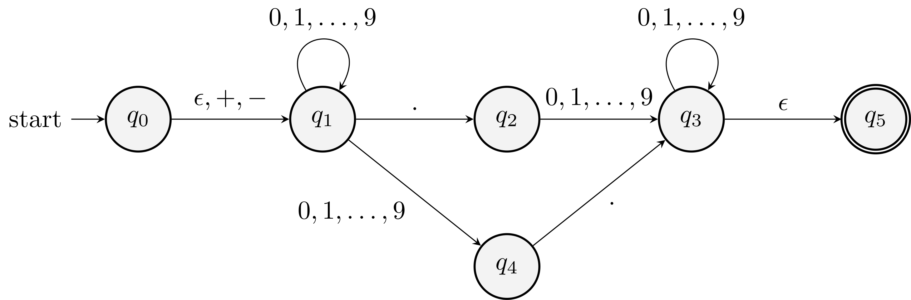
An \(\eps\)-NFA that accepts decimal numbers consisting of:
- An optional \(+\) or \(-\) sign
- A string of digits
- A decimal point
- Another string of digits. Either this string or the string in (2) can be empty.
Compare it with the equivalent DFA.
Formal definition
Compared with the formal definition of NFA, now the transition function \(\delta\) takes a state and a member of \(\Sigma \cup \{ \eps \}\) as input.
\[\begin{equation*} \delta: Q \times (\Sigma \cup \{ \eps \}) \to 2^Q. \end{equation*}\]
Examples
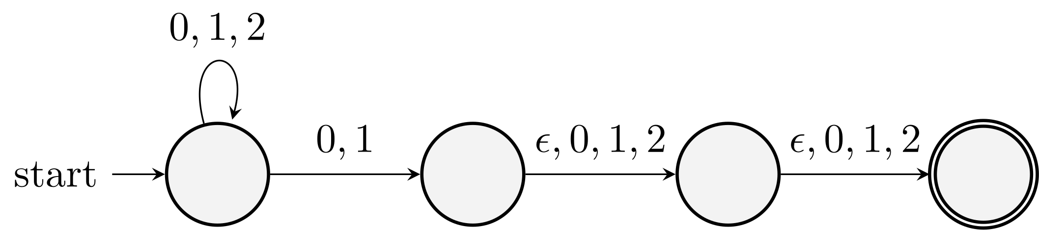
Example. Design \(\eps\)-NFA that accepts all strings over \(\{0,1,2\}\) whose length is at least one and one of the last three letters is not \(2\).
It means that there is a \(0\) or \(1\) in the last three letters.
Example. Design \(\eps\)-NFA that accepts \[\begin{equation*} \begin{split} L = & \{ w \mid w \in \{a,b,c\}^* \land \abs{w}\ge 4 \land\\ & \quad \text{ there is a } bac \text{ in the first five symbols of } w \land\\ & \quad \text{ there is a } acb \text{ in the last five symbols of } w \}. \end{split} \end{equation*}\]
Can you see there are three cases to consider?
Epsilon-closure ECLOSE(\(q\))
The key is to keep track of the possible current states of an automaton.
What is ECLOSE(\(q\)) informally?
Define it yourself.
If \(p, q\) in ECLOSE(\(r\)), do we always have ECLOSE(\(p\)) = ECLOSE(\(q\))? No!
The minimum set such that- \(q \in \text{ECLOSE}(q)\).
- If \(p \in \text{ECLOSE}(q)\) and \(r \in \delta(p, \eps)\), then \(r \in \text{ECLOSE}(q)\).
ECLOSE(\(S\)) is the union of ECLOSE(\(q\)) for \(q \in S\).
Example
- ECLOSE(\(q_0\)) = \(\{q_0, q_1\}\)
- ECLOSE(\(q_2\)) = \(\{q_2\}\)
Extended transition
Take an \(\eps\) move in the end.
Basis: \(w=\eps\), it is ECLOSE(\(q\)).
Induction: \(w=xa\)
- Take the \(x\) transition,
- Take the union with \(a\),
- Take the \(\eps\)-closure.
Eliminate \(\eps\)-transitions
For any \(\eps\)-NFA \(A\), there is a DFA \(B\) equivalent to \(A\). (Not that different from the equivalence of DFA and NFA)
- Compute the ECLOSE.
- Use the subset construction (with ECLOSE after each move)
Often times, you do not need all the subsets! Start from the initial state and generate the subsets one by one.
Example
The DFA obtained by eliminating the \(\eps\)-transitions in Example 2.18 is given in the figure above. For simplicity, the dead state and arrows to it are not shown.
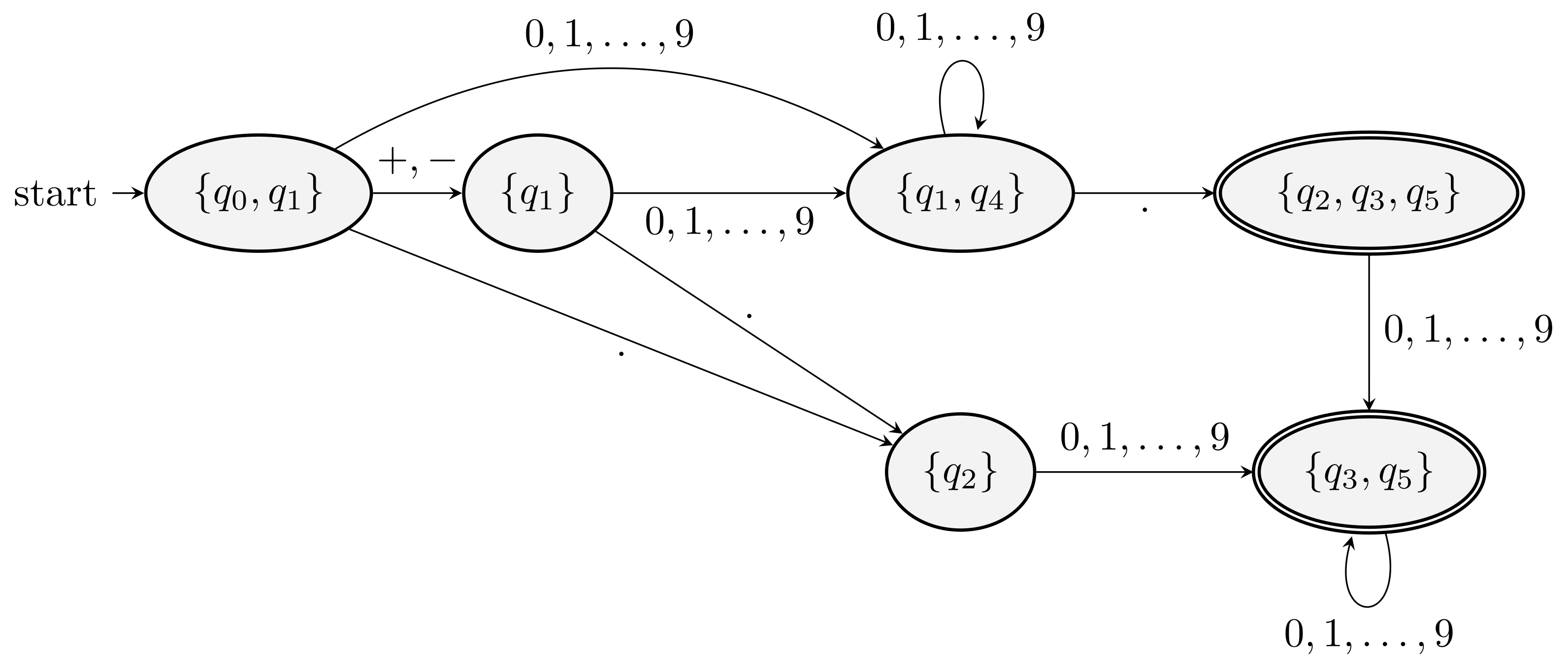
The starting state is \(\text{ECLOSE}(q_0) = \{q_0, q_1\}\).
Regular Expressions
Now we switch our attention from machine-like descriptions of languages—deterministic and nondeterministic finite automata—to an algebraic description of the regular expression.
And show that they can describe all and only regular languages (languages accepted by finite automata).
It is a declarative way to express the strings we want to accept.
grep, lex
Regular expressions: Definition
- Basis: three parts
The constants \(\eps\) and \(\emptyset\) are regular expressions. \(L(\eps) = \{\eps\}\).
If \(a\) is a symbol, then \(a\) is a RE. \(L(a) = \{a\}\).
- Induction: four parts
- If \(E\) and \(F\) are RE, then so is the union \(E + F\). \(L(E+F)=L(E) \cup L(F)\).
- …, then so is the concatenation \(EF\). \(L(EF) = L(E)L(F)\).
- …, then so is the closure \(E^*\). \(L(E^*) = (L(E))^*\).
- …, then so is (E). \(L((E)) = L(E)\).
Examples
01 means \(\{01\}\)
01* means \(\{0, 01, 011, 0111, \ldots\}\)
(01)^* means \(\{\eps, 01, 0101, \ldots\}\)
Example. Write a RE for strings with alternating 0's and 1's.
\((01)^* + (10)^* + 1(01)^* + 0(10)^*\)
or
\((\eps + 1)(01)^*(\eps + 0)\)
Example. Write a RE for binary strings whose first and last letters are the same.
\(0(0+1)^*0 + 1(0+1)^*1 + 0 + 1\)
Example. Write a RE for binary strings where every pair of neighboring 0's occur before every pair of neighboring 1's.
Strings in the language can be partitioned into two parts where the left part has no 11, and the right part has no 00.
\((10 + 0)^* (\eps + 1)(01 + 1)^* (\eps + 0)\)
Precedence of regular expression operators
\(xy+z\)
Order: star, dot, union
Application of RE
Read Section 3.3 of the textbook.
Unix extension
The ability of name and refer to previous strings that have matched a pattern.
More about a way of writing RE succinctly.
- dot . stands for any character
- \([a_1 a_2 \cdots a_k]\) stands for \(a_1 + a_2 + \cdots + a_k\)
- range form [A-Za-z0-9]
- [:digit:], …
Notation
- | is used instead of +
- ? zero or one (\(R? = \eps + R\))
- + one or more (\(R^+ = RR^*\))
- {\(n\)} \(n\) copies of
Lexical analysis
else                   {return (ELSE);}
[A-Za-z][A-Za-z0-9]*   {code to enter the found identifier to the symbol table; return (ID);}
>=                     {return (GE);}
Finding patterns in text
Most editors support RE search and replacement.
Finite Automata and Regular Expression
Define exactly the same set of languages.
Perhaps the most important result in FA & RE.
DFA to RE
Kleene construction
Induction + Restrict the size + Consider expressions between multiple states
Probably the first non-trivial proof we see in this course.
Consider several languages together.
Idea: Roughly, we build expressions that describe sets of strings that label certain paths in the DFA's transition diagram. However, the paths can pass through only a limited subset of the states. In an inductive definition of these expressions, we start with the simplest expressions that describe paths that are not allowed to pass through any states. And inductively build the expressions that let the paths go through progressively larger sets of states.

Proof outline
Let the states be \(\{1, 2, \ldots, n\}\).
Let \(R^{(k)}_{ij}\) be the strings such that if we start from \(i\), we will end up at \(j\) visiting intermediate (not including \(i,j\)) states \(\le k\).
Basis: \(k = 0\). Since all states are numbered \(1\) and above, the restriction on the path is that the path must have no intermediate states at all.
There are two cases to consider.
- An arc from \(i\) to \(j\).
- A path of length \(0\) that consists of state \(i\) only.
If \(i \ne j\), then only case 1 is possible.
In that case, \(R^{(0)}_{i,j}\) is \(a_1 + a_2 + \cdots + a_k\) where there are transitions from \(i\) to \(j\) on symbols \(a_1, a_2, \ldots, a_k\).
If \(i = j\), consider all the loops from \(i\) to itself.
\[\begin{equation*} R^{(0)}_{ij} = \begin{cases} \eps & \text{no self loop},\\ \eps + a_1 + \cdots + a_k & \text{loops with } a_1, \ldots, a_k \end{cases} \end{equation*}\]
Induction: (on \(k\))
The path does not go through state \(k\) at all.
The path goes through state \(k\) at least once.
\[\begin{equation*} R^{(k)}_{ij} = R^{(k-1)}_{ij} + R^{(k-1)}_{ik} \bigl(R^{(k-1)}_{kk}\bigr)^* R^{(k-1)}_{kj}. \end{equation*}\]
The method works even for NFA.
Example
Convert the DFA in the figure to a RE.
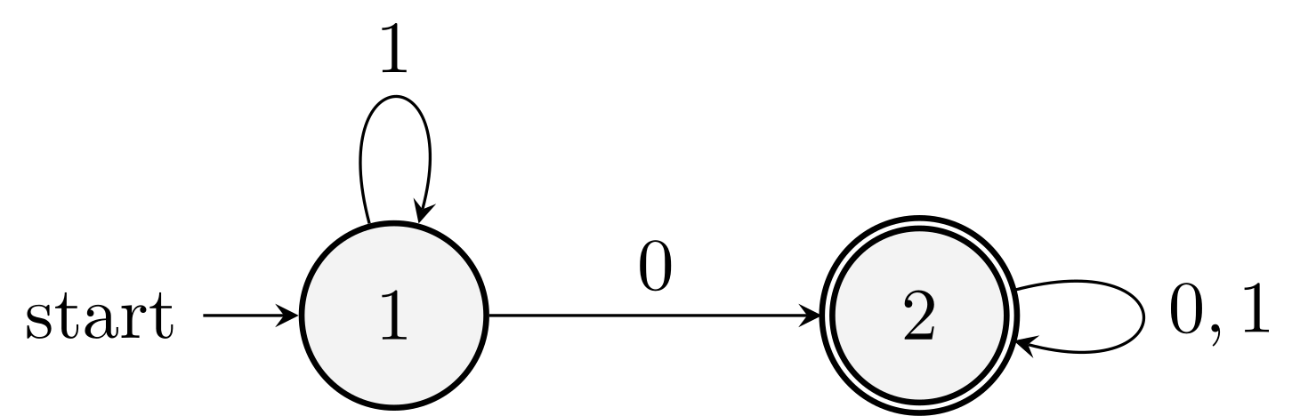
Some intermediate expressions are shown in the table.
Regular Expression \(R^{(0)}_{22}\) \(\eps + 0 + 1\) \(R^{(1)}_{12}\) \(1^*0\) \(R^{(1)}_{22}\) \(\eps + 0 + 1\) \(R^{(2)}_{12}\) \(1^*0(0+1)^*\)
Lecture 4: Finite Automata and Regular Expression
State Elimination Method
Converting DFA's to RE by eliminating states
- Issues for the above method:
- About \(n^3\) intermediate expression.
- The length of the expression could grow as \(4^n\) for an \(n\)-state automaton.
- Each \(R^{(k-1)}_{kk}\) was written in about \(n^2\) expressions.
Idea
The approach to constructing regular expressions we shall now learn involves eliminating states. When we eliminate a state \(s\) all the paths that went through \(s\) no longer exist in the automaton.
Automata with RE as labels!
The eliminating method
Eliminate a state \(s\)
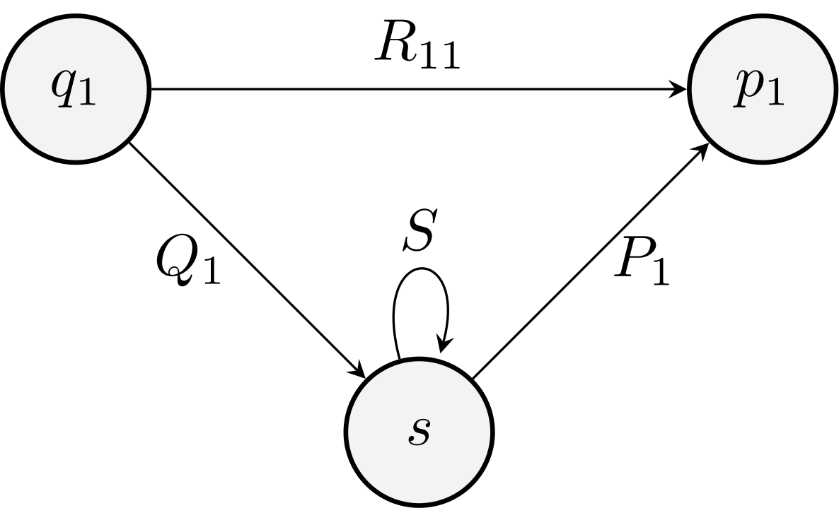
\(R_{11} + Q_1 S^* P_1\)
After the elimination, We will get a two-state or one-state automaton:
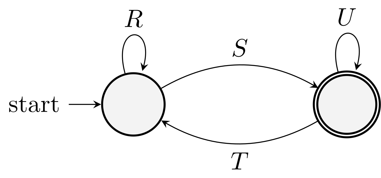
\((R+SU^*T)^*SU^*\)
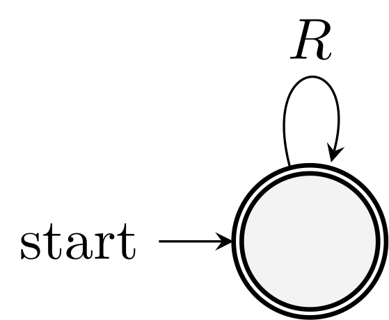
\(R^*\)
State elimination procedure:
- For each accepting state \(q\), eliminate all but \(q\) and \(q_0\).
- Take the union.
Example (Example 3.6 of the textbook)
An automaton accepts all strings whose second or third position from the end has a \(1\).
Step 1. Use RE as labels.
Step 2. Eliminate B. A to C is empty, \(1 \emptyset^* (0+1)\)
Then we branch (for all accepting states)
- First, consider those strings accepted at D. We eliminate C.
- Second, consider those strings accepted at C. We eliminate D. There is no arc added.
Final answer
\((0+1)^*1(0+1) + (0+1)^*1(0+1)(0+1)\)
From RE's to Automata
The language \(L(R)\) of RE \(R\) is also \(L(E)\) for some \(\eps\)-NFA \(E\).
Thompson method
Structural induction on \(R\).
Simplification: \(E\) satisfies the following three extra conditions:- Exactly one accepting state
- No arcs into the initial state
- No arcs out of the accepting state
(Note: 2 and 3 are used to avoid extra discussions in \(R^*\) construction)
Basis: Automata for accepting \(\eps\), \(\emptyset\), \(a\) satisfying the three extra conditions.
Induction: \(R+S\), \(RS\), \(R^*\).
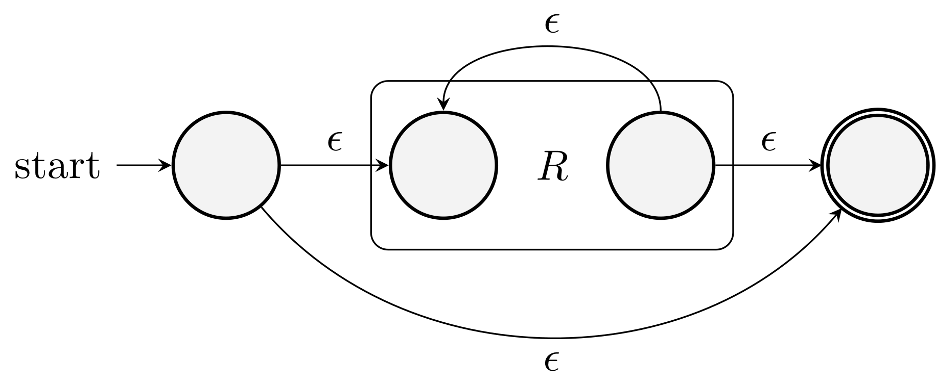
See Figure 3.17 of the textbook for the full construction.
Example. Convert the regular expression \(1(0+1)^*\) to an \(\eps\)-NFA.
Algebraic Laws for RE
What is algebraic law
In mathematics
\(1 + 2 = 2 + 1\) vs \(x + y = y + x\)
Commutativity: The equality holds for all values of the variables \(x\) and \(y\)
Algebra: addition and multiplication
Algebraic laws for RE
Language \(L\) as the variables.
Union as the addition.
Concatenation as multiplication.
Associativity and commutativity
\((L+M)+N = L+(M+N)\)
\(L+M = M+L\)
\((LM)N = L(MN)\)
But not \(LM = ML\).
Identities and annihilators
\(\emptyset + L = L\), identity for addition
\(\eps L = L \eps = L\), identity for concatenation
\(\emptyset L = \emptyset\), annihilator for concatenation
Distributive laws
Let \(L, M, N\) be regular expressions. It holds that \(L(M+N) = LM + LN\).
How to prove it? By definition and set equality.
First, we prove \(L(M+N) \subseteq LM + LN\). For all \(w \in L(M+N)\), there is a partition \(w = w_1w_2\) such that \(w_1 \in L\) and \(w_2 \in M+N\). Case 1, \(w_2 \in M\), \(w \in LM\). Hence \(w \in LM + LN\). Case 2, \(w_2 \in N\), \(w \in LN\). Hence \(w \in LM + LN\).
Second, we prove \(LM + LN \subseteq L(M+N)\).
Idempotent law for union
\(L + L = L\)
Laws involving closures
\((L^*)^* = L^*\), any concatenation of concatenations is a concatenation
\(\emptyset^* = \eps\),
\(\eps^* = \eps\)
\(L^+ = LL^*\)
\(L^* = L^+ + \eps\)
Discovering laws for regular expressions
There is an infinite variety of laws about regular expressions that might be proposed!
Is there a general methodology for finding and proving algebraic laws for RE?
The truth of a law reduces to the equality of two specific languages
Example: \((L+M)^* = (L^*M^*)^*\)
We can specialize the RE operators to act on symbols, one symbol for each language.
- Think of variable \(L\) as a symbol \(a\), \(M\) as \(b\), we get \((a+b)^*\)
- Test if \((a+b)^* = (a^*b^*)^*\)
Main theorem
Theorem (3.13). (A lemma that defines \(L(E)\) alternatively) Let \(E\) be a RE with variables \(L_1, \ldots, L_m\). Let \(C\) be the corresponding concrete RE with symbols \(a_1, \ldots, a_m\). Then, for any instance languages \(S_1, \ldots, S_m\) of \(L_1, \ldots, L_m\), every string \(w\) in \(L(E)\) can be written \(w = w_1 \ldots w_k\), where each \(w_i\) is in one of the language \(S_{j_i}\), and the string \(a_{j_1} \ldots a_{j_k}\) is in the language \(L(C)\). Less formally, we can construct \(L(E)\) by starting with each string \(a_{j_1} \ldots a_{j_k}\) in \(L(C)\) and replacing \(a_{j_i}\) with a string in \(S_{j_i}\).
The intuitive meaning of the theorem is that, starting with a string in the concrete language, you can generate all and only the strings in \(L(E)\) by expanding each symbol into a string from the corresponding language associated with that symbol.
Structural induction on \(E\).
Basis. \(E\) is either \(\eps\), \(\emptyset\), or variable \(L\). If \(E\) is \(L\). \(L(E) = L\) and the concrete expression \(C\) is \(a\), a symbol corresponding to \(L\). Easy.
Induction. If \(E\) is the union, concatenation, or closure, we need to prove the claim.
Suppose \(E = F + G\). Let \(C\) and \(D\) be the concrete expressions of \(F\) and \(G\). Consider \(w \in L(E)\), then \(W\) is either in \(L(F)\) or \(L(G)\). Using induction hypothesis, \(w\) can be obtained by replacing symbols of strings in either \(L(C)\) or \(L(D)\). Hence, \(w\) can be generalized from a concrete string in \(L(C+D)\).
Similarly for \(E = FG\) and \(E= F^*\).
It is a simple method to test a law.
Theorem. \(L(E) = L(F)\) for all choices of languages \(L_1, L_2, \ldots, L_m\) in \(E\) and \(F\) if and only if \(L(C) = L(D)\) where \(C\) and \(D\) are the concrete RE's of \(E\) and \(F\).
The proof is simple and given in Theorem 3.14.
In the only if direction, use the singlet languages. In the other direction, use Theorem 3.13.
Example. \((L+M)^* = (L^*M^*)^*\) and \(L+ML \ne (L+M)L\).
Caveat
The method may become invalid if we add other operators (other than union, concatenation, closure)
Consider \(L \cap M \cap N = L \cap M\). It is obviously false, but \(\{a\} \cap \{b\} \cap \{c\} = \{a\} \cap \{b\}\).
Lecture 5: Pumping Lemma and Properties of Regular Languages
What we will discussion in the next two lectures:
- Proving that a language is not regular.
- Closure properties of RL.
- Finite automata equivalence checking.
- Minimize an automata.
Pumping Lemma
Not every language is regular.
We have proved this using the countability argument.
We will now see concrete examples.
Example
\(L_{\text{EQ}} = \{0^n1^n \mid n \ge 1\}\) is not regular.
Note that it is not the concatenation of \(\{0^n \mid n \ge 1\}\) and \(\{1^n \mid n \ge 1\}\).
Pumping lemma
Let \(L\) be a regular language. Then there exists a constant \(n\) (which may depend on \(L\)) such that for every \(w\) in \(L\) such that \(\abs{w} \ge n\), we can break \(w\) into three strings \(x, y, z\) as \(w = xyz\), such that:
- \(y \ne \eps\).
- \(\abs{xy} \le n\).
- For all \(k \ge 0\), \(xy^kz\) is also in \(L\).
Proof
Use pigeonhole principle to argue that one has to visit a state again.
It's like a game between the 'for all' player and 'exist' player
For all \(L\), there is \(n\), for all \(w\) in \(L\), there is a partition such that for all \(k\), …
Examples
\(L_{\text{EQ}}\)
\(L_{\text{PAL}} = \{ w \mid w = w^R\}\)
\(L_{\text{PRIME}} = \{1^p \mid p \text{ is prime}\}\)
Assume to the contrary that \(L_{\text{PRIME}}\) is a regular language.
By the pumping lemma, there is a constant \(n\), such that for all prime \(p \ge n\), we can partition \(1^p\) into three parts \(x, y, z\) with \(y \ne \eps\), such that \(xy^kz \in L_{\text{PRIME}}\). That is, \(p + (k-1) \abs{y}\) is prime for all \(k\). Choose \(k = p+1\), we have a contradiction. So \(L_{\text{PRIME}}\) cannot be regular.
\(L_{\text{SQUARE}} = \{1^{m^2} \mid m \in \mathbb{N} \}\)
Myhill–Nerode theorem
It provides an if and only if condition for a language to be regular.
EXTRA: Check it out yourself if you are interested. Not required for this course.
Closure Properties
Closure properties
The result of certain operation on regular languages is still regular
- Union
- Closure (star)
- Concatenation
- Intersection
- Complement
- Difference
- Reversal
- Homomorphism
- Inverse homomorphism
Union, intersection, complement
Union
There are \(L=L(R)\), \(M=L(S)\) for RE \(R\) and \(S\) respectively. \(L \cup M = L(R+S)\) by the definition of \(+\).
Complement
Let \(A = (Q, \Sigma, \delta, q_0, F)\) be the DFA for the language.
Complement the accepting states. That is, consider \(A' = (Q, \Sigma, \delta, q_0, Q \setminus F)\).
Closure under intersection!
Idea: Finite memory vs states
Suppose we have DFA's \(A\) and \(B\) for languages \(L\) and \(M\) respectively.
How to design a DFA \(C\) for \(L \cap M\)?
It is known as product construction.
Reversal
The reversal of a string \(w=a_1 \cdots a_n\) is the string \(a_n \cdots a_1\), denoted as \(w^R\).
Define \(L^R = \{w^R \mid w \in L\}\).
If \(L\) is regular, so is \(L^R\).
It can be proved easily via either the automata picture or the RE picture.
See extra notes for how to develop a formal proof from scratch using the reversal as an example.
Lecture 6: Closure, Decision, Equivalence, and Minimization
Closure Properties (cont.)
- Union
- Closure (star)
- Concatenation
- Intersection
- Complement
- Difference
- Reversal
- Homomorphism
- Inverse homomorphism
Homomorphism
A string homomorphism is a function on strings that works by substituting a particular string for each symbol.
Example: \(h(0)=000\), \(h(1)=111\), and \(h(w)=h(a_1) \cdots h(a_n)\).
\(h: \Sigma \rightarrow \Gamma^*\)
Proof. Induction using RE in the textbook.
It is also easy to prove using automata.
Inverse homomorphism
Definition
\(h\) induces a map \(\Sigma^* \rightarrow \Gamma^*\).
\(h^{-1}(L)\) is the set of preimages whose homomorphism is in \(L\).
Example (4.15). \(L\) is \((00+1)^*\), \(h(a) = 01\), \(h(b)=10\). Show that \(h^{-1}(L)\) is \((ba)^*\). Equivalently, \(h(w) \in L\) if and only if \(w\) is of the form \(baba\cdots ba\).
(If) Easy.
(Only-if) Consider the four cases if \(w\) starts with \(a\), ends with \(b\), has \(aa\) as a substring, or has \(bb\) as a substring. These will lead to a \(0,1\) string with a single \(0\) and should be excluded.
So the string has to start with \(b\) and end with \(a\) and is alternating between \(a\) and \(b\).
Inverse homomorphism has the closure property
Theorem. If \(L\) is RE, so is \(h^{-1}(L)\).
Not hard—Fig 4.6 of the textbook.
Let \(A = (Q, T, \delta, q_0, F)\) be the DFA for language \(L\). Define \(B = (Q, \Sigma, \gamma, q_0, F)\) where \(\gamma(q, a) = \hat{\delta}(q, h(a))\).
Prove by induction on \(\abs{w}\) that \(\hat{\gamma}(q, w) = \hat{\delta}(q, h(w))\).
Other Closure Properties
Prefix, suffix, substring!
\[\begin{equation*} \text{Prefix}(L) = \{ u \mid \text{ There is } v \in \Sigma^* \text{ such that } uv \in L\}. \end{equation*}\]
One of your homework problems
NOTE (Mark any states that can reach an accepting state as an accepting state).
Example
Prove that \(\{a^i b^j c^k \mid i,j,k \ge 0, j=k \text{ if } i=1\}\) is not regular.
The pumping lemma won't work!
Intersect with \(\{a b^j c^k\}\),
Consider homomorphism \(h(a) = \eps, h(b) = 0, h(c) = 1\).
Decision Properties
Emptiness, membership, equivalence
Conversion among different representations
\(\eps\)-NFA's to DFA's
Time complexity \(O(n^3 2^n)\) where \(n^3\) comes from the computation for reachable states for all \(n\) states. (Assume the size of the alphabet is a constant)
Often, the complexity is much smaller.
Use lazy evaluation of subsets
\(O(n^3 s)\) where \(s\) is the number of states in the resulting DFA.
Automata to RE
Recall (worst-case) complexity is high \(O(n^3 4^n)\).
Both Kleene construction and the state elimination method have the above complexity.
Do not convert NFA to DFA and then to RE, as it could be doubly exponential!
Emptiness of an RL
Easy to do if we are given a RE explicitly
If given as an FA, emptiness reduces to graph reachability and has time complexity \(O(n^2)\) where \(n\) is the number of states.
Membership
Testing membership is easy if we are given a DFA. By running the DFA, we can solve it in time linear in \(\abs{w}\).
Testing membership for NFA, \(\eps\)-NFA, and RE
Time complexity: \(O(\abs{w} n^2)\).
If we are given an NFA, it is more efficient to simulate on an NFA, maintaining the set of states directly.
If we are given an \(\eps\)-NFA, compute successor states and the \(\eps\)-closure.
If we are given an RE of size \(n\), we can convert it to an \(\eps\)-NFA of size at most \(2n\).
Equivalence and Minimization
State equivalence
Test if two states of a single DFA are equivalent.
\(p, q\) are equivalent if \(\hat{\delta}(p,w)\) is an accept state if and only if \(\hat{\delta}(q,w)\) is for all \(w\).
If two states are not equivalent, we say they are distinguishable.
To find equivalent states, we do our best to find pairs of states that are distinguishable.
States we cannot find distinguishable are equivalent.
Table-filling algorithm: Recursive discovery of distinguishable pairs
Basis: If \(p\) is accepting and \(q\) is non-accepting, they are distinguishable.
Induction: Let \(p\) and \(q\) be states such that for some symbol \(a\), \(\delta(p,a)\) and \(\delta(q,a)\) are a pair of known different states, then they are distinguishable.
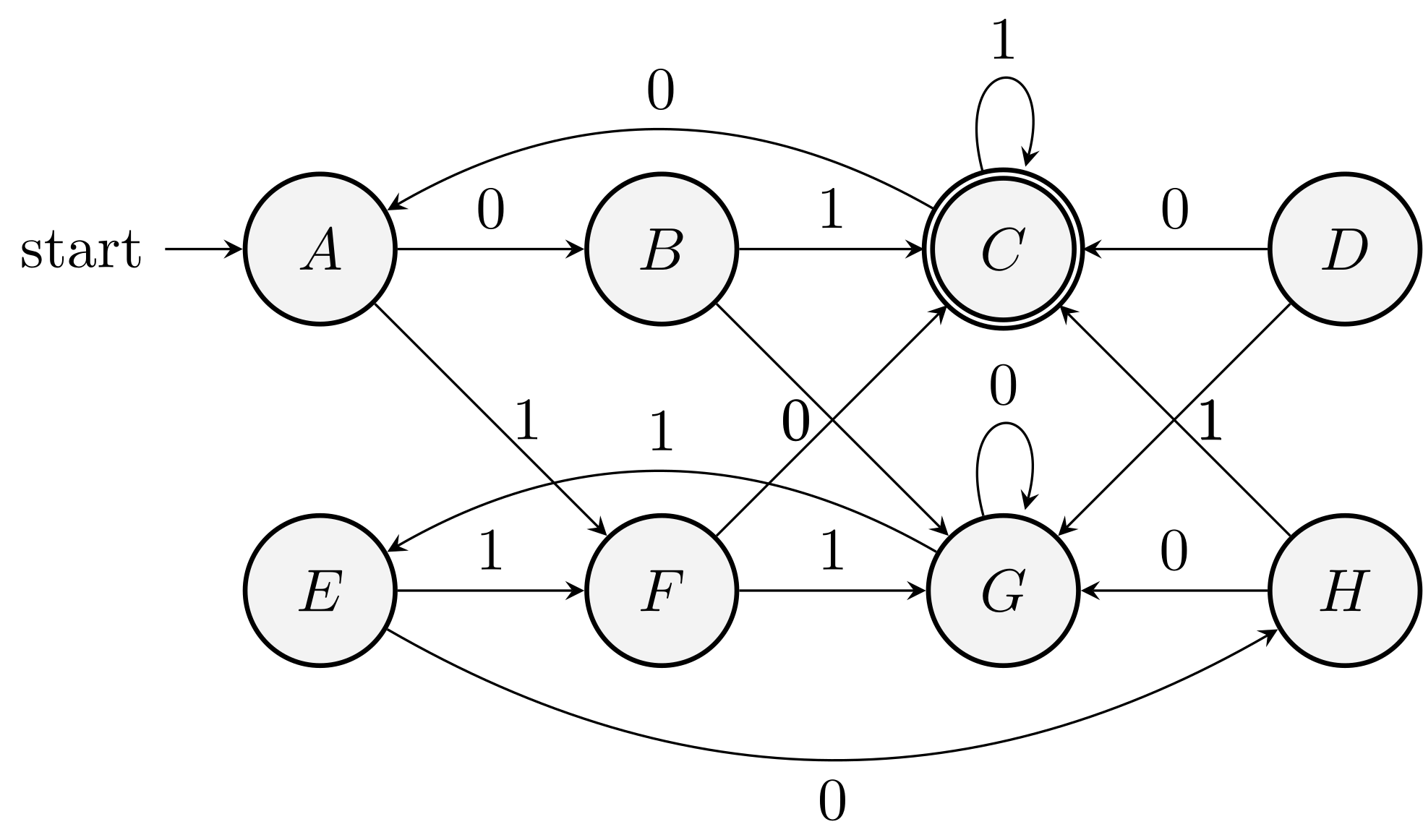
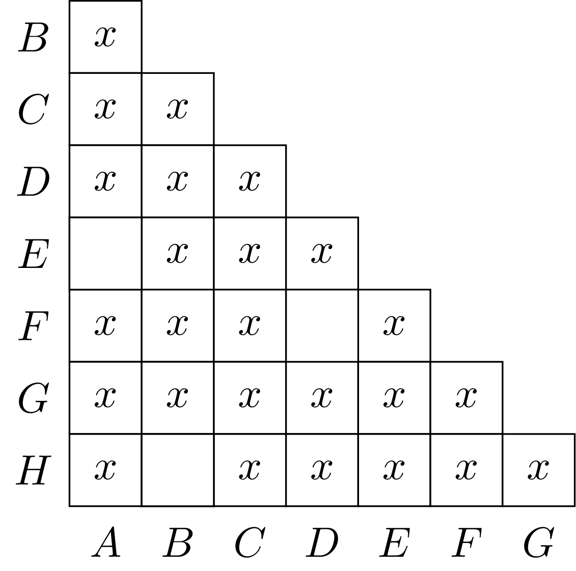
Example (4.18 of the textbook)
Main theorem
Theorem. If two states are not distinguishable by the table-filling algorithm, then they are equivalent.
Assume the theorem is false. That is, there are \(p\), \(q\), distinguishable, but the algorithm does not detect that. Call them bad pairs.
Let \(w\) be one of the shortest strings that distinguish bad pairs. Let the bad pair be \(p\), \(q\).
First, \(w\) cannot be \(\eps\) by the basis of the algorithm. Write \(w = a w'\) and consider \(p' = \delta(p, a)\) and \(q' = \delta(q, a)\).
- If \(p'\) and \(q'\) form a bad pair (distinguishable but not detected). \(w'\) will be a shorter (than w) string that distinguishes a bad pair. Contradiction!
- If \(p'\) and \(q'\) are distinguishable and detected by the algorithm, the induction part of the algorithm will find \(p,q\) distinguishable, and it's contradiction with the fact that \(p,q\) form a bad pair.
- If \(p'\) and \(q'\) are equivalent, \(w\) cannot distinguish \(p\) and \(q\). Contradiction.
As in all possible cases we have a contradiction, our initial assumption is false and the theorem is proved.
There are two important applications of this theorem.
Test equivalence
Put two DFAs together and apply the table-filling algorithm to test if the two start states are equivalent.
Complexity: Easy to show the \(O(n^4)\) bound. We have \(n^2\) pairs, and each will take at most \(O(n^2)\) time.
A careful choice of data structure and analysis shows a \(O(n^2)\) bound. For each pair of states, maintain a list of states that depends on it.
Minimization
- Remove disconnected parts
- Partition the states by equivalence.
Theorem (transitivity). If \(p, q\) are equivalent, \(q, r\) are equivalent, then \(p, r\) are equivalent.
Easy to show. Proof by contradiction.
Use the partitions as states.
It is an equivalence relation (reflexivity, symmetry, transitivity).
Why is it minimal
Let \(M\) be the FA we get from the above. \(N\) is a FA with fewer states accepting the same language.
The starting state of \(M\) and \(N\) are equivalent.
For any state \(p\) in \(M\), there is a \(q\) in \(N\) that are equivalent to \(p\). (Consider a string \(w\) that brings the automaton \(M\) to state \(p\))
Two states in \(M\) are equivalent, a contradiction.
Lecture 7: Context-Free Grammars and Languages
A larger class of languages (CFL) is defined by a natural, recursive notation called CFG.
It is central to compiler technology.
They turned the implementation of parsers from a time-consuming task to a routine job that can be done in an afternoon.
Context-free Grammars (CFG's)
Example
Consider \(L_\text{pal}\) which is the set of binary strings that are palindromes.
Palindrome is not regular.
How to define palindromes?
Basis: \(\eps, 0, 1\) are palindromes.
Induction: If \(w\) is a palindrome, so are \(0w0\) and \(1w1\).
A CFG is a formal notation for expressing such recursive definitions of languages.
A grammar consists of one or more variables that represent languages. In this example, we need only one variable, \(P\).
- \(P \rightarrow \eps\)
- \(P \rightarrow 0\)
- \(P \rightarrow 1\)
- \(P \rightarrow 0P0\)
- \(P \rightarrow 1P1\)
Formal definition
There are four components in a grammatical description of a language:
A finite set of variables.
A finite set of symbols that form the strings of language being defined.
terminals or terminal symbols
A finite set of productions or rules that represent the recursive definition of the language.
One of the variables represents the language being defined. It is called the start symbol.
Each rule consists of:
a. A variable that is being (partially) defined by the production. Often called the head.
b. A production symbol \(\rightarrow\).
c. A string of zero or more terminals and variables. It is called the body.
A CFG is a \(G=(V,T,P,S)\).
Example
\(G_\text{pal} = (\{P\}, \{0,1\}, A, P)\)
Example II
A CFG that represents (a simplification of) expressions in a typical programming language.
\(+\), \(*\), Identifier consists of \(a, b, 0, 1\) only
- \(E \rightarrow I\)
- \(E \rightarrow E + E\)
- \(E \rightarrow E * E\)
- \(E \rightarrow (E)\)
- \(I \rightarrow a\)
- \(I \rightarrow b\)
- \(I \rightarrow Ia \,|\, Ib \,|\, I0 \,|\, I1\)
\(G = (\{E, I\}, T, P, E)\)
\(T\) is \(\{+, *, (, ), a, b, 0, 1\}\)
Derivations of CFG
There are two ways to infer that a particular string is in the language: body to head (recursive inference) and head to body (derivation).
Derivation \(\Rightarrow\)
\(\alpha A \beta\), \(\alpha\) and \(\beta\) are strings in \((V \cup T)^*\) and \(A\) is in \(V\). Let \(A \rightarrow \gamma\) be a rule. Then we say \(\alpha A \beta \Rightarrow \alpha \gamma \beta\).
One derivation step replaces any variable anywhere in the string to the body of one of its production rule.
\(\Rightarrow^*\) zero or more steps of derivation.
Example:
\[\begin{equation*} \begin{split} E & \Rightarrow E * E \Rightarrow I * E \Rightarrow a * E \\ & \Rightarrow a * (E) \Rightarrow a * (E + E) \Rightarrow a * (I + E) \\ & \Rightarrow a * (a + E) \Rightarrow a * (a + I) \Rightarrow a * (a + I0) \\ & \Rightarrow a * (a + b0) \end{split} \end{equation*}\]
Recursive inference vs. derivation.
Leftmost and rightmost derivations
To restrict the number of choices we have in deriving a string.
In each step of leftmost derivations, we replace the leftmost variable in derivations.
\(\Rightarrow_{\text{lm}}\)
\(E \Rightarrow_{\text{lm}} a * (a + b0)\)
\(A \Rightarrow^* w\) if and only if \(A \Rightarrow^*_{\text{lm}} w\)
\(A \Rightarrow^* w\) if and only if \(A \Rightarrow^*_{\text{rm}} w\)
The language of a grammar
- \(L(G) = \{w \in T^* \mid S \Rightarrow^* w\}\)
Theorem. \(L(G_\text{pal})\) is the set of palindromes over \(\{0,1\}\).
What to prove?
(If) \(w\) is a palindrome implies that \(P \Rightarrow^* w\). Use an induction on the length of \(w\).
(Only-if) For all \(w\) such that \(P \Rightarrow^* w\), we conclude that \(w\) is a palindrome. Use an induction on the number of steps in the derivation.
Examples
Construct a CFG for \(\{a^n b^m c^m d^n \mid m, n \ge 1\}\).
Inner part is what we are familiar with.
\(D \rightarrow b D c \,|\, bc\).
Outer part has pairs of \(a\) and \(d\).
\(C \rightarrow a C d \,|\, D\).
Need at least one pair of \(a, d\).
\(S \rightarrow a C d\).
The final answer is therefore \[\begin{align*} S & \rightarrow aCd\\ C & \rightarrow aCd \,|\, D\\ D & \rightarrow bDc \,|\, bc. \end{align*}\]
Construct CFG for \(\{a^m b^n \mid m,n\ge 0, m \ne n\}\).
Use \(A \rightarrow aA \,|\, aAb \,|\, \eps\) to get strings with the condition \(m \ge n\).
Use \(S \rightarrow aA\) to get \(m > n\).
Handle the case of \(m < n\) similarly.
The final solution is \[\begin{align*} S & \rightarrow aA \,|\, Bb\\ A & \rightarrow aA \,|\, aAb \,|\, \eps\\ B & \rightarrow Bb \,|\, aBb \,|\, \eps. \end{align*}\]
Construct CFG for \(\{w \mid w \in \{a,b\}^*, \text{occor}(a, w) = \text{occur}(b, w)\}\).
This is hard as \(a, b\) can be in any order.
Say the string starts with \(a\), we know the tail has one more \(b\).
Color the first \(b\) blue where we have one more \(b\) in the tail and partition the tail into three parts.

It is now easy to write down the rules: \[\begin{equation*} S \rightarrow aSbS \,|\, bSaS \,|\, \eps. \end{equation*}\]
It is a homework problem to prove this construction works.
Let \(G\) be a context-free grammar whose terminal set is \(\{a,b\}\) and starting symbol is \(S\). The production rules are
- \(S \rightarrow \eps \,|\, aB \,|\, bA\),
- \(A \rightarrow a \,|\, aS \,|\, bAA\),
- \(B \rightarrow b \,|\, bS \,|\, aBB\).
Prove that \(L(G) = \{w \mid w \in \{a,b\}^*, \text{occor}(a, w) = \text{occur}(b, w)\}\) too.
Idea: Use mutual induction to prove the following:
a. \(S \Rightarrow^* w\) if and only if \(\text{occur}(a, w) = \text{occur}(b, w)\);
b. \(A \Rightarrow^* w\) if and only if \(\text{occur}(a, w) = \text{occur}(b, w) + 1\);
c. \(B \Rightarrow^* w\) if and only if \(\text{occur}(b, w) = \text{occur}(a, w) + 1\).
Chomsky hierarchy
- Type-0
- Language: Recursive enumerable
- Automata: Turing machine
- Production: \(\gamma \rightarrow \alpha\), \(\gamma\) contains a variable
- Type-1
- Context-sensitive
- Linear-bounded automata
- \(\alpha A \beta \rightarrow \alpha \gamma \beta\) with nonempty \(\gamma\)
- Type-2
- Context-free
- Pushdown automata
- \(A \rightarrow \alpha\)
- Type-3
- Regular
- Finite state automata
- \(A \rightarrow a, A \rightarrow a B\)
Parse tree
A tree representation for derivations.
It is the data structure that represents source programs.
Ambiguity
Constructing parse trees
Given a grammar \(G = (V, T, P, S)\).
The parse trees for \(G\) are trees with the following conditions:
- Each interior node is labeled by a variable in \(V\).
- Each leaf is labeled by either a variable, a terminal or \(\eps\). However, if the leaf is labeled \(\eps\), it must be the only child of its parent.
- If an interior node is labeled \(A\), and its children are labeled \(X_1, X_2, \ldots, X_k\), then \(A \rightarrow X_1 \cdots X_k\) is a production of \(G\).
Example
Parse tree for the derivation of \(I + E\) from \(E\).
The yield of a parse tree
The string of leave contents from left to right.
The yield is what can be derived from the root.
An important case:
- The yield is a terminal string.
- The root is labeled by the start symbol.
Inference, derivations, and parse trees
See Section 5.2 of the textbook for details.
The following are equivalent
- The recursive inference procedure determines that terminal string \(w\) is in the language of variable \(A\).
- \(A \Rightarrow^* w\).
- \(A \Rightarrow^*_{\text{lm}} w\).
- \(A \Rightarrow^*_{\text{rm}} w\).
- There is a parse tree with root \(A\) and yield \(w\).
Proof technique: equivalence.
\(5 \rightarrow 3 \rightarrow 2 \rightarrow 1 \rightarrow 5\)
\(5 \rightarrow 4 \rightarrow 2 \rightarrow 1 \rightarrow 5\)
\(1\rightarrow 5\): Induction on the number of steps used to infer that \(w\) is in the language of \(A\).
Basis: One step. \(A\rightarrow w\). Construct the parse tree directly.
Induction. Suppose \(w\) is inferred after \(n+1\) steps and suppose that for all \(x\) and \(B\) such that the membership of \(x\) in \(B\) was inferred using \(n\) or fewer steps satisfies the theorem. The last step uses a rule \(A\rightarrow X_1 \cdots X_k\). We can break \(w\) into \(w_1 \cdots w_k\) such that
- If \(X_i\) is a terminal, …
- If \(X_i\) is a variable, …
\(5\rightarrow 3\): Let \(G=(V,T,P,S)\) be a CFG, and suppose there is a parse tree with root variable \(A\) and yield \(w \in T^*\). Then there is a leftmost derivation \(A \Rightarrow^*_{\text{lm}} w\) in grammar \(G\).
Induction on the depth of the parse tree. Induction in induction.
\[\begin{equation*} A \Rightarrow^*_{\text{lm}} w_1 w_2 \cdots w_i X_{i+1} \cdots X_k \end{equation*}\]
\(3\rightarrow 2\): trivial.
\(2\rightarrow 1\): Induction on the length of the derivation \(A \Rightarrow^* w\). \(A \Rightarrow X_1 \cdots X_k \Rightarrow^* w\). Then (by proof of induction), we can write \(w = w_1 \cdots w_k\) such that …
Applications of CFG
It is initially discovered by N. Chomsky as a way to describe natural language.
A brief introduction on its uses:
For programming language, CFG provides a mechanical way of turning language descriptions to parse trees. It is one of the first ways in which theoretical ideas in CS found their way into practice.
XML, DTD in XML is essentially a CFG.
Example: html documents (formatting of text).
<html><head></head><body></body></html>
It becomes possible to define and parse the structured documents formally.
Ambiguity
The assumption: a grammar uniquely determines a structure for each string in its language.
That is not always the case.
Sometimes, we can redesign the grammar. Sometimes, we cannot! (inherently ambiguous)
\(E + E * E\) has two derivations from \(E\). The difference is significant.
But sometimes, there are different derivations without significant consequences:
- \(E \Rightarrow E + E \Rightarrow I + E \Rightarrow a + E \Rightarrow a + I \Rightarrow a + b\)
- \(E \Rightarrow E + E \Rightarrow E + I \Rightarrow I + I \Rightarrow I + b \Rightarrow a + b\)
Ambiguity is caused not by the multiplicity of derivations but by the existence of two or more parse trees.
Definition. A CFG is ambiguous if there is a \(w \in T^*\), which has two different parse trees, each with root label \(S\) and yield \(w\). Otherwise, the grammar is unambiguous.
Removing ambiguity
There is no algorithm to tell if a grammar is ambiguous or not (Theorem 9.20)!
There are CFLs that have nothing but ambiguous grammars!
In most practical applications, it is possible to remove ambiguity.
Two causes of ambiguity:
- The precedence of operators is not respected.
- A sequence of identical operators can group either from the left or right.
In the expression example (Example II):
- A factor is an expression that cannot be broken apart by any adjacent operator, either \(+\) or \(*\). In this case, identifier and \(()\).
- A term is an expression that cannot be broken apart by \(+\).
- An expression is any possible expression.
\(I \rightarrow a \,|\, b \,|\, Ia \,|\, Ib \,|\, I0 \,|\, I1\)
\(F \rightarrow I \,|\, (E)\)
\(T \rightarrow F \,|\, T * F\)
\(E \rightarrow T \,|\, E + T\)
It is unambiguous and generates the same language.
Key idea: Create different variables, each representing different binding strengths.
Another example
Dangling else problem: \(S \rightarrow \eps \,|\, iS \,|\, iSeS\) is ambiguous
\(iie\) does not tell us which if statement the else statement referees to.
When the first \(S\) in \(iSeS\) has less \(e\) than \(i\), there will be ambiguity as we don't know which \(i\) the \(e\) is paired with.
The following grammar matches the else with the closest if statement
- \(S \rightarrow \eps \,|\, iS \,|\, iMeS\),
- \(M \rightarrow \eps \,|\, iMeM\).
Derivations are not necessarily unique, even if the grammar is unambiguous. Yet leftmost/rightmost derivations are.
For grammar \(G=(V,T,P,S)\), and string \(w \in T^*\), \(w\) has two distinct parse trees if and only if \(w\) has two distinct leftmost derivations from \(S\).
Proof. Easy. Find the first place where the difference happens.
Example of an inherently ambiguous language
Consider language \(L = \{a^nb^nc^md^m \,|\, m,n\ge 1\} \cup \{a^nb^mc^md^n \,|\, m,n\ge 1\}\) and a CFG for \(L\) \[\begin{align*} S & \rightarrow AB \,|\, C\\ A & \rightarrow aAb \,|\, ab\\ B & \rightarrow cBd \,|\, cd\\ C & \rightarrow aCd \,|\, aDd\\ D & \rightarrow bDc \,|\, bc. \end{align*}\]
We can generate \(a^nb^nc^nd^n\) in two ways. All CFG for this language are ambiguous (see Section 5.4.4 of the textbook).
Lecture 8: Pushdown Automata
Outline
CFLs have a type of automaton that defines them.
Pushdown automata: \(\eps\)-NFA + a stack.
We will consider two types of PDAs, one that accepts by entering an accepting state and one that accepts by emptying its stack.
Definition of a PDA
PDAs can "remember" an infinite amount of information in a restricted manner. (FILO, stack)
Indeed, there are languages that can be recognized by some computer programs (TMs) but not by PDAs.
For example, \(\{0^n1^n2^n \mid n \ge 1\}\) is not a CFL (proved later).
A finite state control, taking inputs and outputs accept/reject while accessing a stack.

Transition of a PDA
In one transition the PDA:
- Consumes an input symbol.
- Goes to a new state.
- Replaces the symbol at the top of the stack by any string. The string could be \(\eps\), where the action corresponds to pop. It could be the same symbol at the top, meaning no change to the stack.
Example of a PDA
\(L_{\text{wwr}}=\{ww^R \mid w \in \{0,1\}^*\}\).
- State \(q_0\), read a symbol, and store it on the stack.
- At any time, we may guess (non-determinism) that we have seen the middle, and go to state \(q_1\).
- In state \(q_1\), we compare input symbols with the symbol at the top of the stack. Pop the stack if they match. Otherwise, this (non-deterministic) branch dies.
- If we empty the stack (or enter accepting state \(q_2\)), we have indeed seen \(ww^R\).
Formal definition
\(P = (Q, \Sigma, \Gamma, \delta, q_0, Z_0, F)\)
States, input symbols, stack symbols, transition function, start state, start symbol (initial stack), accepting states.
\(\delta(q,a,X)\) where \(q\) is a state in \(Q\), \(a\) is either an input symbol or \(\eps\), and \(X\) is a stack symbol.
\(\delta\) outputs a set of pairs \((p, \gamma)\), where \(p\) is the new state, and \(\gamma\) is the string of symbols used to replace the top stack symbol.
Example
The PDA for \(L_{\text{wwr}}\) is \[\begin{equation*} P=(\{q_0, q_1, q_2\}, \{0, 1\}, \{0, 1, Z_0\}, \delta, q_0, Z_0, \{q_2\}). \end{equation*}\]
A graphical notation for PDA's
Similar to transition diagrams for DFA's.
What's new: labels
\(a, X / \gamma\)
\(0, Z_0 / 0Z_0\)
Example (6.2 of the textbook)
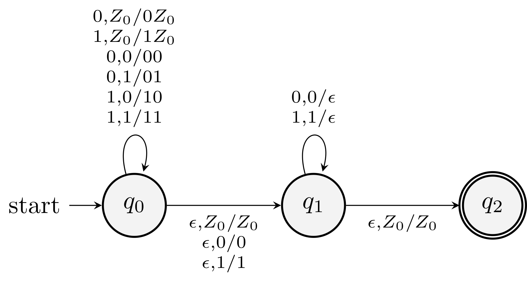
How does it accept \(010010\)?
Instantaneous description of a PDA
Configuration \((q,w,r)\), ID
\(q\): current state
\(w\): remaining input
\(\gamma\): stack content
`turnstile' notation (\(\vdash\) in LaTeX)
Suppose \(\delta(q,a,X)\) contains \((p,\alpha)\). Then for all strings \(w\) in \(\Sigma^*\) and \(\beta\) in \(\Gamma^*\) we write \[\begin{equation*} (q, aw, X\beta) \vdash (p, w, \alpha\beta) \end{equation*}\]
Define \(\vdash^*\) as the reflexive transitive closure of \(\vdash\).
Three important principles about ID's:
- If a sequence of ID's is legal for a PDA \(P\), then the computation formed by adding the same additional input string to the end of the input in each ID is also legal.
- If a computation is legal, then the computation formed by adding the same additional stack symbols below the stack in each ID is also legal.
- If a computation is legal, and some tail of the input is not consumed, then we can remove this tail from the input in each ID, and the resulting computation will still be legal.
Can we remove the tail from the stack?
Theorem. If \((q, x, \alpha) \vdash^* (p, y, \beta)\), then for any string \(w\) in \(\Sigma^*\) and \(\gamma\) in \(\Gamma^*\), it holds that \[\begin{equation*} (q, xw, \alpha\gamma) \vdash^* (p, yw, \beta\gamma). \end{equation*}\]
ASK. Is the converse also true?!
Actually, it is tricky to define the converse; notice the for all quantification. There are strings that a PDA might be able to process by popping its stack, using parts of \(\gamma\). Hence the following converse does NOT hold.
Theorem (Converse candidate). Let \(w\) and \(\gamma\) be any two strings in \(\Sigma^*\) and \(\Gamma^*\) resp. If \[\begin{equation*} (q, xw, \alpha\gamma) \vdash^* (p, yw, \beta\gamma). \end{equation*}\] then \((q, x, \alpha) \vdash^* (p, y, \beta)\).
ASK. What is the difference between converse and contrapositive?
Theorem. If \((q,xw,\alpha) \vdash^* (p,yw,\beta)\), then \((q,x,\alpha) \vdash^* (p,y,\beta)\).
The Language of a PDA
Acceptance by the final state and by empty stack.
Equivalent: In the sense that \(L\) has a PDA that accepts it by state if and only if there is a PDA that accepts it by empty stack.
For a given PDA, however, two acceptance conditions may very likely be different.
Acceptance by final state
\[\begin{equation*} L(P) = \bigl\{w \mid (q_0, w, Z_0) \vdash^* (q, \eps, \alpha) \text{ for some } q \in F \bigr\}. \end{equation*}\]
The PDA in Example (6.2) accepts \(L_{\text{wwr}}\).
Acceptance by empty stack
We do not need to specify \(F\) if empty-stack acceptance is considered.
For each PDA \(P = (Q, \Sigma, \Gamma, \delta, q_0, Z_0)\), define \[\begin{equation*} N(P) = \{w \mid (q_0, w, Z_0) \vdash^* (q, \eps, \eps) \}. \end{equation*}\]
It is easy to change Example 6.2 so that it accepts by empty stack.
Instead of the transition \(\delta(q_1, \eps, Z_0) = \{(q_2, Z_0)\}\), use \(\delta(q_1, \eps, Z_0) = \{(q_2, \eps)\}\).
From empty stack to final state
Proof idea: Use a different initial stack symbol \(X_0\). Push \(Z_0\) as the first step. Whenever we see \(X_0\), pop \(X_0\) and enter the final state.
The full proof is a bit tedious and we omit it in class.
Example. The PDA accepts the if/else errors by empty stack and the transformed PDA that accepts the same language by final state.

From final state to empty stack
Proof idea: For all accepting final state, add \(\eps\) transition to a new state which keeps popping the stack until it's empty.
Is this valid? What could go wrong?!
A PDA that accepts by final state may accidentally empty its stack and we need to use a new initial stack symbol.
Use a new initial stack symbol to solve the problem. The construction is illustrated in the following figure.
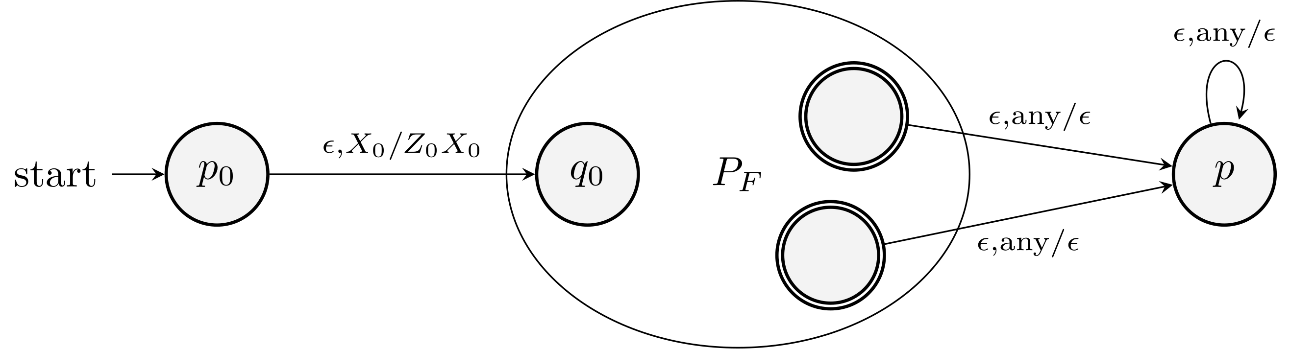
Theorem. Let \(P_F\) be a PDA that accepts by final state. There is a PDA \(P_N\) such that \(L(P_F) = N(P_N)\).
Write the proof yourself and compare it with the textbook.
Step 1. Formally define \(P_N\). Step 2. Prove it works.
Examples
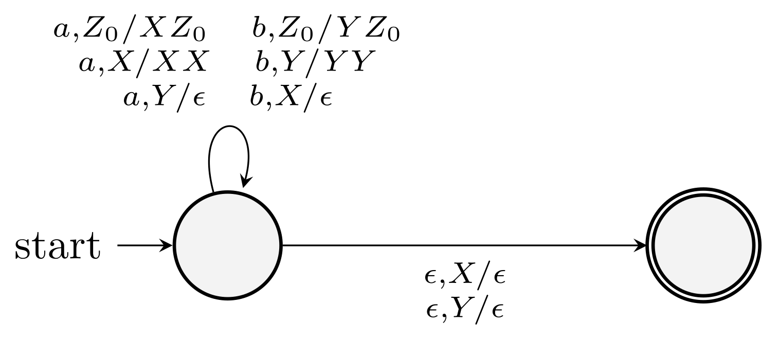
Construct a PDA that accepts \(L = \{ w \in \{a,b\}^* \mid \text{count}(a,w) \ne \text{count}(b,w) \}\).
Use two stack symbols \(X\) and \(Y\) in addition to \(Z_0\).
For \(a\) and \(X\), push \(X\). For \(a\) and \(Y\), pop \(Y\).
For \(b\) and \(X\), pop \(X\). For \(b\) and \(Y\), push \(Y\).
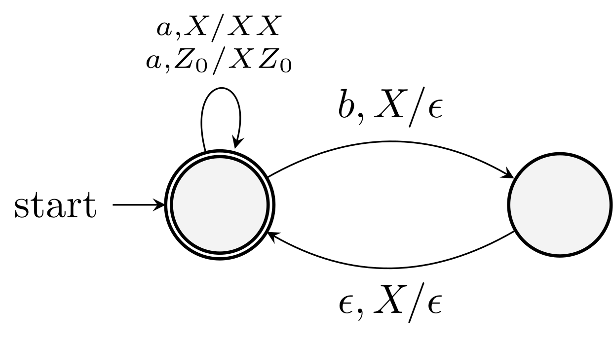
Construct a PDA that accepts strings over \(\{a,b\}\) such that the number of \(a\) is at least twice the number of \(b\) in any prefix of the string.
Consider the accepting state variant.
Push \(X\) for \(a\) and pop \(X\) for \(b\). Use \(\eps\)-move to implement the "twice" condition.
Lecture 9: Equivalence of PDA and CFG
Equivalence of PDA's and CFG's
We will prove that CFG's and PDA's accepting by empty stack are equivalent.
From grammars to PDA's
Consider a left sentential form of the grammar.
Left sentential form is a string in \((V \cup T)^*\) leftmost derivable from \(S\).
Write the left sentential form as \(xA\alpha\). We call \(A\alpha\) the tail.
If the sentential form contains terminals only, its tail is \(\eps\).
We put the tail on the stack with \(A\) at the top.
\(x\) is the consumed input.
So if \(w=xy\), then \(y\) is the remaining input.
Idea: Suppose the PDA is in ID \((q, y, A\alpha)\), representing left-sentential form \(xA\alpha\). It guesses the production rule to use next, \(A \rightarrow \beta\). Enter ID \((q, y, \beta\alpha)\). If there are any terminals appearing at the beginning of \(\beta\alpha\), pop it.
How many states do we need in the above construction?
More formally, we have \[\begin{equation*} P = (\{q\}, T, V \cup T, \delta, q, S), \end{equation*}\] where \(\delta\) is defined by:
- For each variable \(A\), \[\begin{equation*} \delta(q, \eps, A) = \{ (q, \beta) \mid A \rightarrow \beta \text{ is a production of } G \}, \end{equation*}\]
- For each terminal \(a\), \[\begin{equation*} \delta(q, a, a) = \{ (q, \eps) \}. \end{equation*}\]
Theorem. If PDA \(P\) is constructed from CFG \(G\) as above, then \(N(P) = L(G)\).
Proof
We prove that \(w \in N(P)\) if and only if \(w \in L(G)\).
(If) Suppose \(w\) is in \(L(G)\). Then \(w\) has a leftmost derivation
\(S = \gamma_1 \Rightarrow_{\text{lm}} \gamma_2 \Rightarrow_{\text{lm}} \cdots \Rightarrow_{\text{lm}} \gamma_n = w\). We prove that for all \(i\), \((q,w,S) \vdash^* (q, y_i, \alpha_i)\), where \(y_i\) and \(\alpha_i\) form a representation of the left-sentential form \(\gamma_i\). That is, \(\alpha_i\) is the tail of \(\gamma_i\), \(\gamma_i = x_i \alpha_i\), and \(w=x_i y_i\).
Basis: Easy.
Induction: Prove \((q, w, S) \vdash^* (q, y_{i+1}, \alpha_{i+1})\) assuming the \(i\)-th hypothesis.
(Only If) It is the hard part. We want to prove that if \((q,w,S) \vdash^* (q,\eps,\eps)\), then \(S \Rightarrow^* w\).
Strengthen it to all (non-starting) variables and we prove that \[\begin{equation*} \text{If } (q,x,A) \vdash^* (q,\eps,\eps), \text{ then } A \Rightarrow^* x. \end{equation*}\]
Induction on the number of moves taken by the PDA.
Basis. Easy. The only possibility is that \(A \rightarrow \eps\) is used in the PDA.
Induction. Suppose the first move of the PDA corresponds to the production \(A \rightarrow Y_1 \cdots Y_k\).
The PDA needs to pop \(Y_1, \ldots, Y_k\) sequentially. More formally \((q, x_i x_{i+1} \cdots x_k, Y_i) \vdash^* (q, x_{i+1} \cdots x_k, \eps)\) for all \(i\). By induction hypothesis, \(Y_i \Rightarrow^* x_i\).
Write \(x=x_1 \cdots x_k\) where \(x_1\) is the input consumed until \(Y_1\) is popped off from the stack and so on.

From PDA's to grammars
This is non-trivial to prove.
We have seen a very special form of PDA with one state that mimics the derivation of a CFG.
But now, the PDA may be more general.
The special PDA either matches the input and terminals or simulates a rule by the typical change of the stack.
The variables are those symbols that are not simply matched.
The general PDA also has state transitions. What should be the variables in the grammar?
- Net popping of some symbol \(X \in \Gamma\) from the stack.
- A change in state from some \(p\) at the beginning to \(q\) when \(X\) has finally been replaced by \(\eps\).
Understand how the PDA works locally using a collection of moves.
We represent such a variable by the composite symbol \([pXq]\). (It is one single variable)
Theorem (6.14 of the textbook): Let \(P =(Q, \Sigma, \Gamma, \delta, q_0, Z_0)\) be a PDA. Then there is a CFG \(G\) such that \(L(G) = N(P)\).
We construct grammar \(G = (V, T, R, S)\) as follows.
- There is a special symbol \(S\), the start symbol.
- All symbols of the form \([pXq]\) where \(p, q\in Q\) and \(X\in \Gamma\).
The production rules:
For all states \(p\), there is a production rule \(S \rightarrow [q_0Z_0p]\).
Why for all \(p\)?: \([q_0Z_0p]\) is intended to generate all strings \(w\) that cause \(P\) to net pop \(Z_0\) while going from \(q_0\) to \(p\). With acceptance by empty state, we allow all \(p\).
Let \(\delta(q, a, X)\) contain the pair \((r, Y_1 \cdots Y_k)\), where
- \(a\) is either a symbol in \(\Sigma\) or \(a = \eps\).
- \(k\) can be any number, including \(0\), where the pair is \((r, \eps)\).
Then for all list of states \(r_1, \ldots, r_k\), \(G\) has rule
\[\begin{equation*} [qXr_k] \rightarrow a[rY_1r_1][r_1Y_2r_2] \cdots [r_{k-1}Y_kr_k]. \end{equation*}\]
This is the key construction. It is special in the sense that it only contains one terminal in each rule.
Intuition: one way to net pop \(X\) and go from state \(q\) to \(r_k\) is to read \(a\), then use some input to pop \(Y_1\) off the stack while going from state \(r\) to state \(r_1\), then pop \(Y_2\) and transit from \(r_1\) to \(r_2\), and so on.
Claim: \([qXp] \Rightarrow^* w\) if and only if \((q, w, X) \vdash^* (p, \eps, \eps)\)
Proof.
(If) Suppose \((q, w, X) \vdash^* (p, \eps, \eps)\). We need to show \([qXp] \Rightarrow^* w\).
Induction on the number of steps made by the PDA.
Basis. Easy. If there is one step, \((p, \eps)\) is in \(\delta(q, a, X)\) and \(a=w\).
Induction. Suppose \[\begin{equation*} (q, w, X) \vdash (r_0, x, Y_1 \cdots Y_k) \vdash^* (p, \eps, \eps), \end{equation*}\] takes \(n\) steps in total.
We have \(w=ax\) where \(a\) could be a symbol or \(\eps\).
The PDA will need to net pop \(Y_1, \ldots, Y_k\) sequentially while consuming \(w\).
To include \(w\) in the language, the grammar needs to simulate the above procedure using derivations.
Let the state after the net popping of \(Y_1\) be \(r_1\), …
The first step above implies that \((q, a, X)\) contains \((r_0, Y_1 \cdots Y_k)\) and by our construction, \(G\) has a rule \[\begin{equation*} [qXp] \rightarrow a[r_0Y_1r_1][r_1Y_2r_2] \cdots [r_{k-1}Y_kp] \end{equation*}\]
Note that the net popping of \(Y_i\) will have less steps and the induction hypothesis applies.
(Only-If) If \(S \Rightarrow^* w\), then \(w \in N(P)\).
Induction on the number of steps in the derivation.
Basis. One step. \([qXp] \rightarrow w\) must be a production.
By the construction of the grammar, this is a production rule only if
- \(w = a\)
- \((p, \eps)\) is in \(\delta(q, a, X)\).
Induction. Suppose \[\begin{equation*} [qXr_k] \Rightarrow a[r_0Y_1r_1] \cdots [r_{k-1}Y_kr_k] \Rightarrow^* w. \end{equation*}\]
The first derivation means that \(\delta(q, a, X)\) contains \((r_0, Y_1 \cdots Y_k)\).
Write \(w = a w_1 \cdots w_k\) and \([r_{i-1}Y_ir_i] \Rightarrow^* w_i\). Use induction hypothesis.
(The principles of extending the remaining input and stack will be used.)
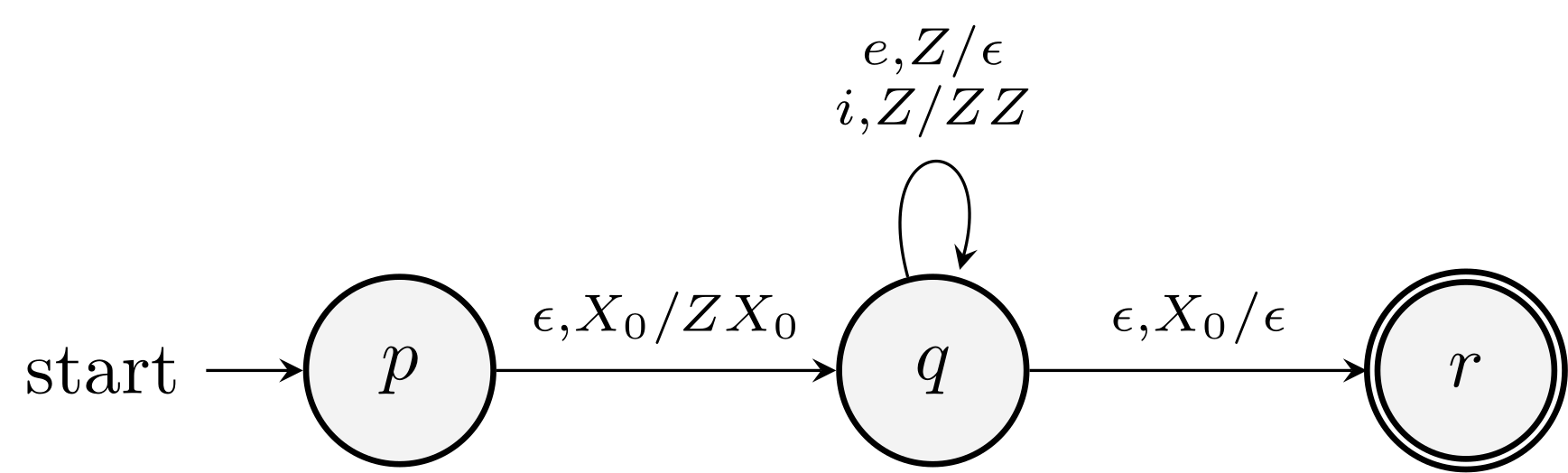
Example
Convert PDA \(P = (\{q\}, \{i, e\}, \{Z\}, \delta, q, Z)\) to a grammar (PDA in Example 6.10).
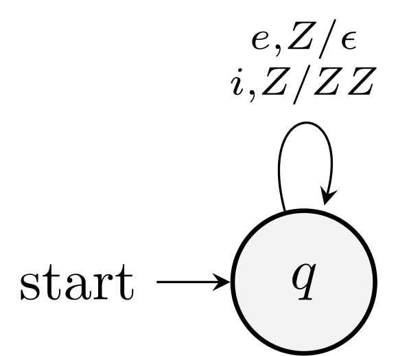
\(S \rightarrow [qZq]\)
As \(\delta(q, i, Z)\) contains \((q, ZZ)\), we get production \([qZq] \rightarrow i [qZq] [qZq]\). In this simple example, we have one such rule, if the PDA had \(n\) states, we would need \(n^2\), as the middle two and the last \(q\) should run over all possible states.
As \(\delta(q, e, Z)\) contains \((q, \eps)\), we get production \([qZq] \rightarrow e\).
Rename \([qZq]\) as \(A\), we have
- \(S \rightarrow A\)
- \(A \rightarrow i A A | e\)
As \(S\) and \(A\) derive the same language, we can write the grammar as \(S \rightarrow iSS | e\).
Deterministic PDA
PDA is by definition non-deterministic.
In this part, we study a deterministic variant of PDA's.
Useful for modeling parsers.
Definition
- A PDA is deterministic if
- For all \(q, a, X\), \(\delta(q, a, X)\) is empty or a singleton.
- If there is a \(a \in \Sigma\) such that \(\delta(q, a, X)\) is not empty, then \(\delta(q, \eps, X)\) must be empty.
Properties
DPDA's accept languages that is between RL's and CFL's.
Theorem. Any regular language has a DPDA.
There is a non-regular language (say, \(L_\text{wcwr}\)) accepted by DPDA. So DPDA's are more powerful than FA's.
\[\begin{equation*} L_{\text{wcwr}} = \bigl\{ wcw^R \mid w \in \Sigma^* \bigr\} \end{equation*}\]
However, DPDA's with empty stack acceptance are quite weak.
Theorem. A language \(L\) is in \(N(P)\) for some DPDA \(P\) if and only if \(L\) has the prefix property (no two strings \(x, y\in L\) and \(x\) is the prefix of \(y\)) and \(L\) is \(L(P')\) for some DPDA \(P'\).
DPDA's are weaker than PDA's.
Examples
\(L_\text{wcwr}\) does have the prefix property.
\(L(0^*)\) is regular but does not have prefix property.
\(L_\text{wwr}\) cannot be accepted by any DPDA's (even with final-state acceptance).
Proof idea: Suppose \(P\) has seen \(n\) \(0\)'s and then sees \(110^n\). It must verify that there were \(n\) \(0\)'s after the \(11\) and to do so it must pop its stack. So the PDA will not be able to act differently for two cases of further remaining inputs \(0^n110^n\) (should accept as \(w=0^n110^n\)) and \(0^m110^m\) (should reject if \(m\ne n\)).
DPDA and Ambiguity
Languages accepted by DPDA's are unambiguous.
Yet DPDA languages are not exactly the subset of CFL's that are not inherently ambiguous. (Example \(L_{\text{wwr}}\)).
Theorem. If \(L = N(P)\) for some DPDA \(P\), then \(L\) has an unambiguous CFG.
The construction we used for PDA to CFG will lead to unambiguous CFG. Note that \(\delta(q, a, X) = \{(r, Y_1 \cdots Y_k) \}\) may lead to multiple productions in \(G\). But as \(P\) is deterministic, only one will be consistent with what \(P\) actually does.
Theorem. If \(L = L(P)\) for some DPDA \(P\), then \(L\) has an unambiguous CFG.
Endmarker trick. Treat \(\$\) as a new variable and add \(\$ \rightarrow \eps\)!
Summary of Languages Studied

Lecture A: Properties of Context-Free Languages
Normal Forms for CFG
Chomsky Normal Form
Every CFL (without \(\eps\)) has a CFG whose rules have the form \(A\rightarrow BC\) or \(A\rightarrow a\).
Some preliminary simplifications:
- Eliminate useless symbols, variables or terminals that do not appear in any derivation of a terminal string.
- We must eliminate \(\eps\) productions, those of the form \(A \rightarrow \eps\).
- We must eliminate unit productions, those of the form \(A \rightarrow B\).
Eliminating useless symbols
What symbols do not appear in any derivation of a terminal string?
What is your suggestion? Reachability?
Example: Consider the grammar
- \(S \rightarrow AB \,|\, ab\)
- \(A \rightarrow a\)
\(X\) is useful for a grammar \(G\) if there is some derivation of the form \(S \Rightarrow^* \alpha X \beta \Rightarrow^* w\).
So, in addition to reachability from \(S\), we also require \(X\) to be generating, that is \(X \Rightarrow^* w\) for some \(w\).
If we (1) eliminate symbols not generating and then (2) those not reachable, we will (proved after) have only useful symbols left.
The order matters. Consider the example above.
\[\begin{equation*} G \overset{\text{(1)}}{\longrightarrow} G_2 \overset{\text{(2)}}{\longrightarrow} G_1. \end{equation*}\]
Theorem (7.2). Let \(G\) be a CFG such that \(L(G) \ne \emptyset\). Let \(G_2\) be the grammar obtained by eliminating symbols not generating. Let \(G_1\) be the grammar obtained by eliminating symbols not reachable from \(G_2\). Then \(G_1\) has no useless symbols, and \(L(G_1) = L(G)\).
Suppose \(X\) is a symbol that remains in \(G_1\). We know \(X \Rightarrow^*_G w\) for some w. Since all symbols involved in this derivation are generating, we have \(X \Rightarrow^*_{G_2} w\). Since \(X\) is not eliminated in the second step, we know that \(S \Rightarrow^*_{G_2} \alpha X \beta\). Since every symbol used in this derivation is reachable, we have \(S \Rightarrow^*_{G_1} \alpha X \beta\), showing \(X\) is reachable in \(G_1\).
As \(\alpha X \beta\) contains only symbols in \(G_2\), which are generating by definition, we have \(\alpha X \beta \Rightarrow^*_{G_2} xwy\). This means that all symbols in \(xwy\) are reachable from \(S\). Thus, this derivation is also a derivation of \(G_1\). So \(S \Rightarrow^*_{G_1} \alpha X \beta \Rightarrow^*_{G_1} xwy\), and \(X\) is generating in \(G_1\).
It is easy to show \(L(G) = L(G_1)\) and we omit the proof.
Finding generating and reachable symbols
Both are easy; we use finding generating symbols as an example.
Basis: All symbol in \(T\) is generating.
Induction: If \(A \rightarrow \alpha\) is a production rule, and all symbol in \(\alpha\) is generating, then so is \(A\). This rule includes \(A \rightarrow \eps\).
This works as 1) all symbols found this way are generating, and 2) all generating symbols can be found in this way.
Eliminating \(\eps\)-productions
We will show \(\eps\)-productions are not essential.
Theorem. If \(L\) has a CFG, then \(L - \{ \eps \}\) has a CFG without \(\eps\)-production.
A variable \(A\) is nullable if \(A \Rightarrow^* \eps\).
If \(A\) is nullable and appears in a production body of, say, \(B \rightarrow CAD\), we add a rule \(B \rightarrow CD\) alongside \(B \rightarrow CAD\) (do not allow \(A\) to derive \(\eps\)).
Find nullable symbols iteratively.
Basis. If \(A \rightarrow \eps\) is a rule, then \(A\) is nullable.
Induction. If there is a rule \(B \rightarrow C_1 \cdots C_k\) and each \(C_i\) is nullable, then \(B\) is nullable.
Theorem. The above procedure finds all the nullable symbols.
Eliminating \(\eps\)-productions.
First, find all nullable variables. For a rule \(A \rightarrow B_1 \cdots B_k\) if \(m\) of the \(k\) variables are nullable, consider \(2^m\) replicates of the rule removing all possible combinations of the nullable variables.
There is one exception when \(m=k\) as we don't include the case when all variables are \(\eps\). And we do not keep any \(A \rightarrow \eps\).
Example
Consider grammar
- \(S \rightarrow AB\)
- \(A \rightarrow aAA \,|\, \eps\)
- \(B \rightarrow bBB \,|\, \eps\)
Resulting grammar
- \(S \rightarrow AB \,|\, A \,|\, B\)
- \(A \rightarrow aAA \,|\, aA \,|\, a\)
- \(B \rightarrow bBB \,|\, bB \,|\, b\)
Proof
The proof is a bit tedious. Inductively prove a stronger statement:
\[\begin{equation*} A \Rightarrow^*_{G_1} w \text{ iff } A \Rightarrow^*_G w \text{ and } w\ne \eps. \end{equation*}\]
Eliminate unit productions
Productions like \(A \rightarrow B\) where \(B\) is a variable.
Unit pairs: \((A, B)\) such that \(A \Rightarrow^* B\) uses unit productions only.
Computation of unit pairs.
Basis. \((A, A)\) is a unit pair for all \(A \in V\).
Induction. \((A, B)\) is a unit pair, and \(B\rightarrow C\) is a production, then \((A, C)\) is a unit pair.
Claim: The above procedure computes all unit pairs.
Eliminate unit productions:
- Compute all unit pairs
- For all unit pairs \((A, B)\), if \(B \rightarrow \alpha\) is not a unit production, add \(A \rightarrow \alpha\) to \(G_1\).
- Add all non-unit productions of \(G\) to \(G_1\)
Example
- \(S \rightarrow A\)
- \(A \rightarrow 0BD \,|\, 0B\)
- \(B \rightarrow 0BC \,|\, 1\)
- \(C \rightarrow 1\)
Unit pairs \((A,A)\), \((B,B)\), \((C,C)\), \((D,D)\), \((S,S)\) and \((S,A)\)
After elimination, we have
- \(S \rightarrow 0BD \,|\, 0B\)
- \(A \rightarrow 0BD \,|\, 0B\)
- \(B \rightarrow 0BC \,|\, 1\)
- \(C \rightarrow 1\)
CFG simplification
- Eliminate \(\eps\)-productions
- Eliminate unit productions
- Eliminate useless symbols
Again, the order matters!
Theorem (7.14). If \(G\) is a CFG that generates a language that contains at least one string other than \(\eps\), then there is another CFG \(G_1\) such that \(L(G_1) = L(G) - \{\eps\}\) and \(G_1\) has no \(\eps\)-production, unit production, or useless production.
Chomsky Normal Form
Every nonempty CFL without \(\eps\) has a grammar \(G\) in which all productions are in one of two simple forms, either:
- \(A \rightarrow BC\) where \(A,B,C\) are variables;
- \(A \rightarrow a\) where \(a\) is a terminal.
Furthermore, \(G\) has no useless symbols.
Such a grammar is said to be in Chomsky Normal Form.
Easy to do given Theorem 7.14.
Arrange that all bodies of length 2 or more consist only of variables
Break bodies of length 3 or more into a cascade of productions, each with a body consisting of two variables.
\(A \rightarrow B_1 C_1\), \(C_1 \rightarrow B_2 C_2\), …, \(C_{k-2} \rightarrow B_{k-1} B_k\).
The Pumping Lemma for CFL
Again, it is a tool for showing that certain language is not a CFL.
Size of a parse tree
Theorem (7.17). Suppose we have a parse tree for a grammar of CNF and suppose the yield is \(w\). If the length of the longest path is \(n\), we have \(\abs{w} \le 2^{n-1}\).
Proof. Easy.
Pumping lemma
Let \(L\) be a CFL. There is a constant \(n\) such that if \(z\) is any string in \(L\) of length at least \(n\), then we can write \(z=uvwxy\), satisfying
- \(\abs{vwx} \le n\), that is the middle part is not too long.
- \(vx \ne \eps\).
- For all \(k\ge 0\), \(uv^kwx^ky \in L\).

Suppose a CNF of \(L\) has \(m\) variables. Choose \(n = 2^m\).
What's the smallest possible length of the longest path? \(m+1\).
By the pigeonhole principle, we have \(A_i = A_j\) for \(l-m \le i < j \le l\).
REMARK: Note that \(k\) in the lemma can be \(0\) , and that condition 1 of the lemma follows from Theorem 7.17.
Application
Examples: Show that the following languages are not CFL.
- \(\{0^n1^n2^n \mid n \ge 1\}\).
- \(\{0^i1^j2^i3^j \mid i, j \ge 1\}\).
- \(\{ww \mid w \in \{0,1\}^*\}\).
Example 1.
Assume to the contrary that it is a CFL. Let \(n\) be the number promised by the pumping lemma. Then consider string \(0^n1^n2^n\) which is of length greater than \(n\). There is a partition of the string into \(uvwxy\) such that \(\abs{vwx} \le n\), \(vx \ne \eps\), and \(uv^iwx^iz\) is in the language.
As the middle part \(vwx\) has length at most \(n\), we know that \(v\) and \(x\) cannot have both \(0\) and \(2\). So when we take \(i > 1\), the number of \(0\) and \(2\) will not be the same in \(uv^iwx^iy\).
Closure Properties of CFL's
What are operations on CFL that are guaranteed to produce a CFL?
Similar to what we proved for RL, with some differences.
CFL's are closed under the three RE operations, homomorphism, inverse homomorphism.
CFL's are not closed under intersections or differences. Yet the intersection or difference of a CFL with a RL is always CFL.
Substitutions
For every \(a \in \Sigma\) we choose a language \(L_a\) which is over a possibly different alphabet. Define \(s(a) = L_a\) for all \(a\in \Sigma\).
If \(w = a_1 a_2 \cdots a_n\) is a string in \(\Sigma^*\), then \(s(w)\) is the language concatenating \(L_{a_1}, \ldots, L_{a_n}\).
We further extend the definition to \(s(L)\) as the union of \(s(w)\) for all \(w \in L\).
Theorem (7.23). If \(L\) is CFL and \(s(a)\) is a CFL for each \(a \in \Sigma\), then \(s(L)\) is a CFL.
Consider the parse tree. Replace terminal \(a\) of \(G\) for \(L\) with new start symbol \(S_a\).

Caveat: Use different variables in all grammars involved.
Application of the substitution theorem
CFL is closed under:
- Union (\(\{1, 2\}\))
- Concatenation (\(\{12\}\))
- Closure (\(^*\)) and positive closure (\(^{+}\))
- Homomorphism
Reversal
Reversal of all production rule.
CFL's are not closed under intersection
Example (7.26): \(L_1 = \{0^n1^n2^i\}\) and \(L_2 = \{0^i1^n2^n\}\).
How did we prove that RL is closed under intersections?
Product construction: we simulate two machines simultaneously. But we only have one stack!
Intersection with RL
A weaker statement we can prove is that the intersection of a CFL and a RL is a CFL.

Caveat: the PDA may take an \(\eps\) move which the DFA won't (DFA will not change the state while the PDA takes an \(\eps\) move).
Set difference and complement
If \(L\), \(L_1\), and \(L_2\) are CFL's and \(R\) is a RL, then
- \(L - R\) is a CFL.
- \(\overline{L}\) is not necessarily CFL.
- \(L_1 - L_2\) is not necessarily CFL.
- \(L-R = L \cap \overline{R}\).
- \(L_1 \cap L_2 = \overline{\overline{L_1} \cup \overline{L_2}}\).
- Take \(L_1 = \Sigma^*\).
Inverse homomorphism

Suppose \(h\) applies to symbols of alphabet \(\Sigma\) and produces strings in \(T^*\).
\(L\) is a language over \(T\) and PDA \(P = (Q,T,\Gamma,\delta, q_0, Z_0, F)\) accepts \(L\) by final state. We construct a new PDA \[\begin{equation} P' = (Q', \Sigma, \Gamma, \delta', (q_0, \eps), Z_0, F \times \{\eps\}) \end{equation}\] where:
- \(Q'\) is the set of all pairs \((q,x)\) such that: a. \(q\) is a state in \(Q\) and, b. \(x\) is a suffix of some string \(h(a)\). (Save buffer in the state)
- \(\delta'\) is defined by the following rules: a. \(\delta'((q,\eps), a, X) = \bigl\{ \bigl((q, h(a)), X\bigr) \bigr\}\). b. If \(\delta(q, b, X)\) contains \((p, \gamma)\), where \(b \in T\) or \(b = \eps\), then \(\delta'((q,bx), \eps, X)\) contains \(((p,x), \gamma)\).
- Start with an empty buffer.
- Accept with empty buffer and final state.
Claim. \((q_0, h(w), Z_0) \vdash^*_P (p, \eps, \gamma)\) if and only if \(((q_0,\eps), w, Z_0) \vdash^*_{P'} ((p, \eps), \eps, \gamma)\).
Proof. The proofs in both directions are inductions on the number of moves made by the two automata. In the (If) part, observe that once the buffer of \(P'\) is nonempty, it cannot read another input symbol and must simulate \(P\) until the buffer has become empty.
Decision Properties of CFL's
Very little can be decided about a CFL.
Yet we can decide emptiness and membership.
Complexity of Converting Among CFG's and PDA's
The following are efficient (linear complexity):
- CFG to PDA,
- PDA accepts by final state to and from PDA accepts by empty stack.
Yet, PDA to CFG is not by default.
The following construction induces a cost roughly of order \(n^n\) \[\begin{equation*} [qXr_k] \rightarrow a[rY_1r_1][r_1Y_2r_2] \cdots [r_{k-1}Y_kr_k]. \end{equation*}\]
The solution is to modify the PDA.
We can break the pushing of a long string of stack symbols into a sequence of at most \(n\) steps that each pushes one symbol.
Theorem (7.31). There is an \(O(n^3)\) algorithm that takes a PDA \(P\) whose representation has length \(n\) and produces a CFG of length at most \(O(n^3)\)
Complexity of Converting to Chomsky Normal Form
Theorem (7.32). Given a grammar \(G\) of length \(n\) we can find an equivalent Chomsky normal form grammar for \(G\) in time \(O(n^2)\).
Testing emptiness
We have seen how to do this before.
Check whether \(S\) is generating.
It is easily done in \(O(n^2)\).
We can even do it in time \(O(n)\), using certain simple data structure (See Fig. 7.11 of the textbook, link and count).
Testing membership
Inefficient membership tests are obvious: we simulate all possible non-deterministic choices.
There is a much more efficient algorithm known as the CYK algorithm to test the membership of a CFL, named after Cocke, Younger, Kasami.
Dynamic programming on CFG in Chomsky normal form.
In the CYK algorithm, we construct a triangular table where the horizontal axis corresponds to the positions of the string \(w = a_1 a_2 \cdots a_n\). Entry \(X_{ij}\) is the set \(\bigl\{ A \mid A \Rightarrow^* a_{i} a_{i+1} \cdots a_{j} \bigr\}\).
Work row by row upwards.
\[\begin{equation*} \left. \middle\vert \begin{matrix} X_{14} & & &\\ X_{13} & X_{24} & & \\ X_{12} & X_{23} & X_{34} &\\ X_{11} & X_{22} & X_{33} & X_{44}\\\hline a_1 & a_2 & a_3 & a_4 \end{matrix} \right. \end{equation*}\]
Basis: \(j=i\). If \(A \rightarrow a_i\) is a production, \(A \in X_{ii}\).
Induction. \(j > i\). \(A \in X_{ij}\) if and only if there exists \(k\) such that \(i\le k < j\) and there is \(B \in X_{ik}\), \(C \in X_{(k+1)j}\), and \(A \rightarrow BC\) is a production.
Example (7.34): Consider CNF grammar \(G\) \[\begin{align*} S & \rightarrow AB \,|\, BC\\ A & \rightarrow BA \,|\, a\\ B & \rightarrow CC \,|\, b\\ C & \rightarrow AB \,|\, a \end{align*}\]
Test if \(baaba\) is in the language or not.
\[\begin{equation*} \left. \middle\vert \begin{matrix} \{S,A,C\} & & & &\\ {-} & \{S,A,C\} & & &\\ {-} & \{B\} & \{B\} & &\\ \{S,A\} & \{B\} & \{S,C\} & \{S,A\} &\\ \{B\} & \{A,C\} & \{A,C\} & \{B\} & \{A,C\}\\\hline b & a & a & b & a \end{matrix} \right. \end{equation*}\]
The time complexity is \(O(n^3)\), where \(n\) is the length of the input string and the grammar is fixed as a constant.
Earley parser, which we won't describe here, is more efficient for unambiguous grammars and has \(O(n^2)\) time complexity.
Preview of undecidable CFL problems
- Ambiguity of grammars (Theorem 9.20)
- Inherent ambiguity
- Emptiness of intersection
- Equality
- Equality to \(\Sigma^*\)
Lecture B: Turing Machines
Until now, we have been interested primarily in simple classes of languages and how they can be used for relatively constrained problems.
Now we shall start looking at the question of what languages can be defined by any computational device whatsoever.
We will show that there are specific problems that we cannot solve using a computer (undecidable).
Is It a "Hello World!" Program?
The particular problem we discuss is whether the first thing a C program prints is Hello World!. Although we might imagine that simulation of the program would allow us to tell what the program does, we must in reality contend with programs that take an unimaginably long time before making any output at all. This problem of not knowing when, if ever, something will occur is the ultimate cause of our inability to tell what a program does.
Collatz conjecture
Consider the following program in C.
while (n > 1) {
  n = (n % 2 == 0) ? n/2 : 3*n+1;
}
printf("Hello World!");
The Collatz conjecture states the while loop will terminate for all natural number \(n\).
This is numerically verified for very large \(n\), but remains open. It is an infamous problem that young mathematicians are usually told not to spend time on.
Watch Video on Collatz conjecture.
Is it a Hello World program for all input \(n\)?
Fermat's last theorem
It can be expressed as a hello world program (see Fig 8.2 of the textbook).
Chapter 9 is devoted to undecidability.
Undecidable Problems Must Exist
There are more problems than programs.
The question is whether natural undecidable problems exist.
We will see the Hello World! problem is one.
Turing Machines
The need for a formal definition of computation
For example, we would have great difficulty reducing the hello world problem to the question of whether a grammar is ambiguous if we don't have a definition of computation.
We need an easy way to represent the what it means to compute something.
Hilbert, Gödel, Church, Turing
Why is the Turing machine special among all equivalent models?
Turing machine captures the notion of computation intuitively!
Church-Turing thesis: A function on the natural numbers can be calculated by an effective method if and only if it is computable by a Turing machine.
- \(\lambda\)-calculus
- Recursive functions
- Turing machines
- Conway's game of life
- Wang tiles
- C, Python, Java, …
Formal definition

A Turing machine consists of
- A finite control
- A 1-D tape, divided into cells; each cell can hold a finite number of symbols.
- A head positioned at one of the cells
Formal definition
A TM is a \(7\)-tuple \[\begin{equation*} M = (Q, \Sigma, \Gamma, \delta, q_0, B, F), \end{equation*}\] where the transition function is a partial function such that, if \(\delta(q, X)\) is defined, it is a triple \((p, Y, D)\).
Initial configuration:
Input is a finite-length string over the input alphabet; it is placed on the tape. All other cells, extending indefinitely to the left and right, hold the blank symbol. The head is positioned at the left-most cell of the input.
How a TM computes
The transition is a function of the state of the machine, and the tape symbol scanned. In one move, it will
- Change the state.
- Write a symbol in the cell scanned.
- Move the head one cell left or right.
This simple model captures the intuition of what a computation is!
“An algorithm is a finite answer to an infinite number of questions.” — Stephen Kleene
“STUDYING:
You are all computer scientists.
You know what FINITE AUTOMATA can do. You know what TURING MACHINES can do.
For example, Finite Automata can add but not multiply. Turing Machines can compute any computable function. Turing machines are incredibly more powerful than Finite Automata.
Yet the only difference between a FA and a TM is that the TM, unlike the FA, has paper and pencil.
Think about it. It tells you something about the power of writing. Without writing, you are reduced to a finite automaton. With writing you have the extraordinary power of a Turing machine.”, by Manuel Blum
Instantaneous Description for TMs
- Current state \(q\),
- Position of the head,
- Tape content (non-blank portion, and blanks up to the head position).
We use \(X_1X_2 \cdots X_{i-1} q X_i X_{i+1} \cdots X_n\) to represent an ID.
Formal description of a move
As in the PDA case, we use \(\vdash\) to denote a move.
Suppose \(\delta(q,X_i) = (p,Y,L)\), we can write \[\begin{equation*} \begin{split} & X_1 X_2 \cdots X_{i-1} q X_i X_{i+1} \cdots X_n \vdash X_1 X_2 \cdots \\ & \qquad\qquad X_{i-2} p X_{i-1} Y X_{i+1} \cdots X_n. \end{split} \end{equation*}\]
Two exceptions:
- If \(i=1\), then \[\begin{equation*} qX_1 X_2 \cdots X_n \vdash p B Y X_2\cdots X_n, \end{equation*}\]
- If \(i=n\) and \(Y=B\), \[\begin{equation*} X_1 X_2 \cdots X_{n-1} q X_n \vdash X_1 X_2 \cdots X_{n-2} p X_{n-1}. \end{equation*}\]
Right moves are discussed similarly.
Example
A TM that accepts \(\{0^n1^n \mid n\ge 1\}\).
Design: Replace \(0\) with \(X\) and move right until the head sees a \(1\), change it to \(Y\) and move back, …

The computation of the TM on inputs \(0011\) and \(0010\) \[\begin{equation*} \begin{split} & q_0 0011 \vdash Xq_1 011 \vdash X0 q_1 11 \vdash Xq_2 0 Y 1 \vdash\\ & q_2 X 0 Y 1 \vdash X q_0 0 Y 1 \vdash XX q_1 Y 1 \vdash XXY q_1 1 \vdash\\ & XX q_2 YY \vdash X q_2 X YY \vdash XX q_0 YY \vdash\\ & XXY q_3 Y \vdash XXYY q_3 B \vdash XXYYB q_4 B.\\[.5em] & q_0 0010 \vdash^* XXY0 q_1 B. \end{split} \end{equation*}\]
The language of a TM
With \(\vdash\) defined, we can define the language of a TM \(M\) as \[\begin{equation*} L(M) = \{w \mid q_0 w \vdash^* \alpha p \beta \text{ for some } p \in F\}. \end{equation*}\]
The set of languages that can be accepted by a TM is called the recursively enumerable languages or RE languages.
We say a TM halts if it enters a state \(q\) while scanning a tape symbol \(X\) and \(\delta(q, X)\) is undefined.
We assume that a TM always halts when it is in an accepting state.
It is, however, not always possible to require that a TM halts even if it does not accept.
Those languages with Turing machines that do halt eventually, regardless of whether or not they accept, are called recursive languages. Also known as decidable problems.
The collection of recursive languages are denoted \(\mathrm{R}\) and it is known that \(\mathrm{R} \subsetneq \mathrm{RE}\).
Programming a TM
You will see why TMs are as powerful as conventional computers next lecture.
Storage in the state
Store a finite amount of information in the state of the TM.
A machine at state \(q\) and storing \(A,B,C\) can be thought of as a machine with state \([q,A,B,C]\).
Example
Design a TM that accepts \(L(01^* + 10^*)\).
Idea: Remember the first input symbol in the state.
Multiple tracks
Divide the tape into multiple tracks.
A common use is to use a track to hold markers.
Example: Design a TM for \(L_{\text{wcw}} = \{wcw \mid w \in (0+1)^{+} \}\).
We can use \(\{B, *\} \times \{0,1,c,B\}\) as the set of tape symbols.
Here \(*\) is the marker and \([B,X]\) is treated as the tape symbol \(X\) for \(X = 0, 1, c, B\).
The idea using a second track as marker is simple, but the full construction is tedious and consists of fourteen transition rules (See Example 8.7 of the textbook).
Subroutine
A Turing machine subroutine is a set of states that perform some useful process.
This set contains a start state and another state that temporarily has no moves (return state).
The call to the subroutine occurs whenever the machine enters the start state of the subroutine.
As TMs do not have a mechanism to remember a return address, we use copies of the set of states.
Example of Subroutine: Multiplication TM
Task: Design a TM with input \(0^m10^n1\) and output \(0^{mn}\).
Overall strategy
The tape will contain \(0^i 1 0^n 1 0^{kn}\).
In each basic step, we change the first 0 in the first group to \(B\) and add \(n\) 0's to the last group.
Finally, we change the leading \(1 0^n 1\) to blanks.
Subroutine Copy
\(0^{i} 1 q_1 0^n 1 0^{(k-1)n} \vdash^* 0^{i} 1 q_5 0^n 1 0^{kn}\).
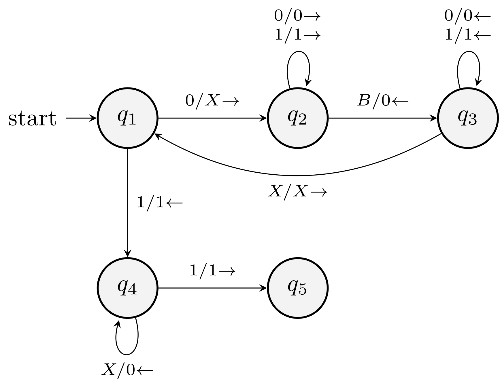
Complete construction
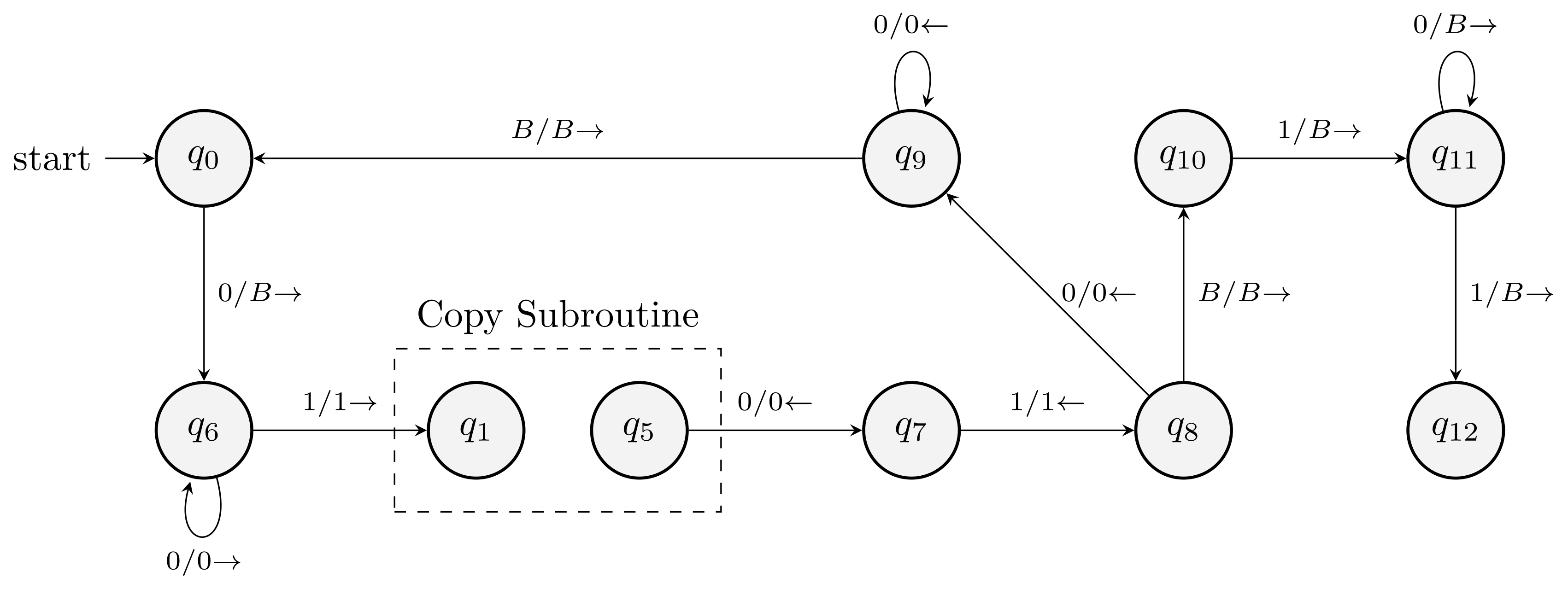
Notice how the copy subroutine is called.
Lecture C: Variants of Turing Machines
Extensions of TMs
There are several natural extensions of TMs that turn out to have the same power as standard TMs.
This stability of TMs is another important reason that we define a Turing machine as it is last lecture.
Multiple tapes
Multitape TMs are variants of TMs that have multiple tapes and multiple read/write heads.
It is impossible to store the head positions in the state of the TM!
Even though after \(n\) moves the number of possible head positions is finite, the set of possible head positions is infinite.
Solution: A move of a multitape TM depends on the state and all tape symbols the heads point to.

Theorem: Every language accepted by the multitape TM is RE.
Use a multi-track construction with marker tracks indicating the head positions.
It is sometimes too complicated to give low level specification of the TMs and so we allow us to informally describe the machine by natural languages.
Perform several left to right sweeping as follows:
Scan from left to right, store the current head symbols in the state.
After the first pass, the machine can compute the new symbols that needs to be written and the movement of each head.
For each track representing a tape, run from the left to the right, write the symbol and change the head marker
Change the state.
Efficiency of the simulation
Let \(T\) be the number of steps the multitape TM runs for some input. The simulation takes \(O(T^2)\) steps, as the standard TM can simulate one move of the multitape TM by sweeping all non-blank symbols on the tape constant number of times.
We should get used to the above high-level description of TMs.
Nondeterministic TMs
In an NTM, \(\delta(q,X)\) is a set of triples (possible moves).
The possible IDs of a NTM forms a computational tree.
A nondeterministic TM accepts if there is at least one accepting branch.
Simulation of NTMs by TMs.
Let \(M_N\) be a nondeterministic TM. Then there is a deterministic TM \(M_D\) such that \(L(M_N) = L(M_D)\).
Proof idea: Use a two-tape machine to run a search algorithm
The first tape maintains a queue of ID's of \(M_N\). Initialize to the initial ID of \(M_N\).
Run breadth-first search on the nondeterministic computation tree.
Each time, take an ID, compute the children of it, add them to the queue.
- Accept whenever the current ID is an accepting state of \(M_N\).
Restricted TMs
Semi-infinite tape
Idea: Fold the tape!

Multistack
A PDA with two or more stacks.
Two stacks can simulate a tape: left and right cells of the head.
First push all input to a stack to simulate the starting situation of the TM (input on the tape).
Counter machines
Two equivalent definitions
- Each counter is a nonnegative integer, and the machine can add or subtract each counter by \(1\). If the counter is already \(0\), it is not possible to subtract by \(1\) from it. The transition of the machine is determined by the state, input symbol, and which of the counters are zero.
- A restricted multistack machine where there are two stack symbols \(X\) and \(Z_0\), \(Z_0\) is initially on each stack, the machine will only replace \(Z_0\) with a string of the form \(X^i Z_0\) for some \(i\ge 0\) and replace \(X\) by \(X^i\) for some \(i\ge 0\).
Three-counter machines are powerful
Theorem. Every RE language is accepted by a three-counter machine.
We begin with a two-stack machine and encode the stack symbols in the following way. Suppose \(r-1\) symbols are used, identified with numbers \(1\) to \(r-1\). We think of the stack \(X_1 X_2 \cdots X_n\) as an integer in base \(r\), so this stack is represented by \(X_nr^{n-1} + X_{n-1} r^{n-2} + \cdots + X_2 r + X_1\).
The third counter works as ancillary space to compute push (\(i \mapsto ir+X\)), pop (\(i \mapsto \lfloor i/r \rfloor]\)), and replacement.
Two-counter machine is powerful
Theorem. Every RE language is accepted by a two-counter machine.
Encode three-stack content \((i,j,k)\) as \(2^i3^j5^k\) and use the other counter as auxiliary working space.
TMs and Computers
Simulating TMs by computers
Easy. But we need to assume that we can add disks to the computer if needed.
See websites that host TM simulators.
Simulating computers by TMs
We start with a realistic but informal model of a typical computer.
- Memory
- The program of the computer is stored in some words of the memory. Indirect addressing is allowed.
- Each instruction involves a limited number of words.
- A typical computer has registers, which are memory words with especially fast access.
A multitape TM simulating a typical computer's instruction cycle:
Search the first tape for an address that matches the instruction number on the second tape.
Decode the instruction (
add, copy, jump).If the instruction requires the value of some address, read the value at the address.
Simulate the execution of the instruction.
If it is not a
jumpinstruction, add \(1\) to the second tape.Theorem (Informal). Under reasonable conditions, the TM can simulate \(n\) steps of the computer in time \(O(n^3)\).

The Busy Beaver TMs (Optional)
TMs are hard to understand compared with FAs and PDAs.
The busy beaver problem will give you a very concrete example of the above claim.
We define an \(n\)-state TM over binary alphabet as a TM where there are \(n\) states \(1, 2, \ldots, n\) and a halting state \(H\). The tape symbol set \(\Gamma = \{0,1\}\) and \(0\) is the blank symbol. The busy beaver function \(\BB(n)\) is defined to be the maximum number of steps an \(n\)-state TM if it will eventually halt (enter state \(H\)) with all-0 input tape.
It is introduced by Tibor Rado in 1962.
Known values
\(n\) \(\BB(n)\) \(1\) \(1\) \(2\) \(6\) \(3\) \(21\) \(4\) \(107\) \(5\) \(47,176,870\) \(6\) ? Allen Brady proved that \(\BB(4)\) equals \(107\) in 1983.
The value of \(\BB(5)\) is determined early 2024 by an international collaborative project called the Busy Beaver Challenge after being an open problem for over 40 years.
\[\begin{equation*} \left. \begin{array}{@{}c@{}} \BB(6) \ge 10^{10^{\cdot^{\cdot^{\cdot^{\scriptstyle 10}}}}} \end{array} \right\rbrace \scriptstyle \text{15 times} \end{equation*}\]
This year (2025), the bound improves to 10,000,000 times.
How many \(n\)-state TMs are there?
\({(4n+4)}^{2n}\), which isn't too bad!
But why is it so hard?!
In order to prove that \(\BB(5) = 47,176,870\), for example, we not only need to construct a TM that runs this many steps, but also need to prove that if a TM runs more than this many steps, it will never stop.
Most tellingly, in 2024 a six-state Turing machine was found that almost corresponds to the Collatz problem. So if one wanted to show that this machine stops (or continues to run forever), this would be tantamount to solving the Collatz problem. (Scientific American)
“If and when artificial superintelligences take over the world, they can worry about the value of \(\BB(6)\). And then God can worry about the value of \(\BB(7)\).”, by Scott Aaronson.
Fun facts about \(\BB(n)\).
Theorem. For any computable function \(f: \mathbb{N} \to \mathbb{N}\), there is a number \(n_f\) such that, \(\BB(n) > f(n)\) for all \(n \ge n_f\).
Theorem. Let \(T\) be a computable and arithmetically sound axiomatic theory. Then there exists a constant \(n_T\) such that for all \(n \ge n_T\), no statement of the form \(\BB(n) = k\) can be proved in \(T\).
Reading
The Quanta Magazine article With Fifth Busy Beaver, Researchers Approach Computation’s Limits tells interesting stories behind the work of identifying the value of \(\BB(5)\).
Scott Aaronson's paper on The Busy Beaver problem.
The Scientific American article on the 5th busy beaver is also an interesting read.
Lecture D: Undecidability
Codes for Turing machines
We can encode Turing machines as binary strings (or integers).
We assume the states are \(q_1, q_2, \ldots, q_r\) for some \(r\) and \(q_1\) is the starting state and \(q_2\) is the only accepting state.
We assume the tape symbols are \(X_1, X_2, \ldots, X_s\) for some \(s\). \(X_1\), \(X_2\), and \(X_3\) will be \(0\), \(1\), and \(B\) respectively.
We refer to direction \(L\) as \(D_1\) and \(R\) as \(D_2\).
If \(\delta(q_i, X_j) = (q_k, X_l, D_m)\), we code this rule by string \(0^i10^j10^k10^l10^m\). A code for the TM \(M\) consists of all the codes for transitions, in some order, separated by a pair of \(1\)'s: \[\begin{equation*} C_1 11 C_2 11 \cdots C_{n-1}11 C_n. \end{equation*}\]
If \(w\) is a binary string, treat \(1w\) as a binary integer \(i\) and call \(w\) the \(i\)-th string. We write the \(i\)-th string as \(w_i\).
We could now define the \(i\)-th TM as the TM for which the \(i\)-th string is one of its codes. If a code is invalid, we assign to it the TM that automatically rejects.
Undecidability
The diagonalization language
Consider a table indexed by \(i\) and \(j\) telling whether \(M_i\) accepts input string \(w_j\).

The diagonalization language is \[\begin{equation*} L_{\text{d}} = \{ w_i \mid w_i \not\in L(M_i) \}. \end{equation*}\]
The diagonalization language is not RE
Theorem. \(L_{\text{d}}\) is not RE. That is, there is no TM \(M\) such that \(L(M) = L_{\text{d}}\).
Proof. Assume to the contrary that there is a TM \(M = M_i\) such that \(L(M_i) = L_{\text{d}}\).
If \(w_i \in L_{\text{d}}\), we have \(w_i \not\in L(M_i) = L_{\text{d}}\). A contradiction.
If \(w_i \not \in L_{\text{d}}\), we have \(w_i \in L(M_i) = L_{\text{d}}\). Again a contradiction.
Recursive vs. recursive enumerable
A language \(L\) is recursive (or decidable) if \(L = L(M)\) for some Turing machine \(M\) such that (a) if \(w \in L\), then \(M\) accepts \(w\) and halts and (b) if \(w \not\in L\), \(M\) eventually halts and never enters an accepting state.
There are languages that are
- Recursive,
- Recursive enumerable but not recursive,
- Not recursive enumerable.
The complements of recursive languages are recursive.
Theorem. If \(L\) is recursive, so is \(\overline{L}\).
Let \(L = L(M)\) such that \(M\) always halts. Run \(M\) and flip the decision.
Theorem. If both \(L\) and \(\overline{L}\) are RE, then \(L\) is recursive.
Let \(L=L(M_1)\) and \(\overline{L} = L(M_2)\). Consider a TM with two tapes. One tape simulates the tape of \(M_1\), and the other simulates the tape of \(M_2\). If \(M_1\) ever accepts, \(M\) accepts, and if \(M_2\) ever accepts, \(M\) halts without accepting.
Thus, on all inputs, \(M\) always halts and \(L = L(M)\).
Example. As \(L_{\text{d}}\) is not RE, \(\overline{L}_{\text{d}}\) is not recursive (but it is in RE).
The universal language
Definition. The universal language \(L_{\text{u}} = \{ (M, w) \mid M \text{ accepts } w\}\).
Theorem There is TM \(U\) (known as the universal TM) such that \(L_{\text{u}} = L(U)\).
We design \(U\) in a similar way as the design of the TM simulating traditional computers. \(U\) is a multitape TM as in the following figure.

The operation of \(U\) can be summarized as follows:
- Examine the validity of the code of \(M\), if invalid, reject (halts without accepting).
- Initialize the string \(w\) on the second tape in some encoded form.
- Place \(0\), the starting state of \(M\), on the third tape.
- To simulate a move of \(M\),
\(U\) searches on its first
tape for a transition \(0^i10^j10^k10^l10^m\) such that \(0^i\) is the state on tape \(3\), \(0^j\) is the tape symbol of \(M\). \(U\) will
- Change state on tape \(3\) to \(0^k\),
- Replace \(0^j\) on tape 2 by \(0^l\); shift-over if needed,
- Move the head on tape 2 accordingly.
- If \(M\) has no transition and halts, \(U\) must do likewise.
- If \(M\) accepts, so does \(U\).
In this way, \(U\) simulates \(M\) on input \(w\) and \(U\) accepts \((M, w)\) if and only if \(M\) accepts \(w\).
von Neumann architecture: stored-program computer.
As we now know there is a universal TM, we can use
Simulate the TM (whose code is on the tape)in our informal description of TMs!Compare with \(L_{\text{PDA}} = \{(P,w) \mid \text{PDA } P \text{ accepts } w \}\).
REMARK: An explicit code for \(U\) is given in The Emperor's New Mind by R. Penrose.
Undecidability of the universal language
Theorem. \(L_{\text{u}}\) is RE but not recursive.
It is RE as \(L_{\text{u}} = L(U)\).
Assume to the contrary that \(L_{\text{u}}\) is recursive. Then we know \(\overline{L}_{\text{u}}\) is also recursive. Let \(M\) be the TM such that \(L(M) = \overline{L}_{\text{u}}\). We will use \(M\) to design a TM \(M'\) that accepts \(L_{\text{d}}\), and this will contradict with the fact that \(L_{\text{d}}\) is not RE.
The TM \(M'\) is defined as follows:
- Given \(w\) on its input, \(M'\) changes the input to \(w111w\).
- \(M'\) simulates \(M\) on the new input. If \(w\) is \(w_i\) in the enumeration of strings, then \(M'\) determines whether \(M_i\) accepts \(w_i\). As \(M\) accepts \(\overline{L}_{\text{u}}\), \(M'\) accepts if and only if \(M_i\) does not accept \(w_i\) (that is, \(w_i \in L_{\text{d}}\)).
The Halting problem
To Halt or Not to Halt, that is the question.
The Halting Problem. One often hears of the halting problem for Turing machines as a problem similar to \(L_u\)—one that is RE but not recursive. In fact, the original Turing machine of A. M. Turing accepted by halting, not by final state. We could define \(H(M)\) for TM \(M\) to be the set of inputs \(w\) such that \(M\) halts given input \(w\), regardless of whether or not \(M\) accepts \(w\). Then, the halting problem is the set of pairs \((M, w)\) such that \(w\) is in \(H(M)\). This problem (language) is another example of one that is RE but not recursive.
Reductions
If we have an algorithm to convert instances of a problem \(P_1\) to instances of a problem \(P_2\) that have the same answer, then we say that \(P_1\) reduces to \(P_2\).

If \(P_1\) is not recursive, then \(P_2\) cannot be recursive.
If \(P_1\) is not RE, then \(P_2\) cannot be RE.
Formally, a reduction from \(P_1\) to \(P_2\) is a Turing machine that takes an instance of \(P_1\) written on its tape and halts with an instance of \(P_2\) on its tape.
We can prove undecidability using reductions!
Turing machines accepting the empty language
We regard strings as TMs they represent.
Consider two languages:
- \(L_{\text{e}} = \{ M \mid L(M) = \emptyset \}\)
- \(L_{\text{ne}} = \{ M \mid L(M) \ne \emptyset \}\)
Theorem. \(L_{\text{ne}}\) is RE but not recursive.
We can construct a TM (non-deterministic) \(M\) such that \(L(M) = L_{\text{ne}}\) as follows. \(M\) takes as input a TM code \(M_i\) and guesses (or enumerates deterministically) an input \(w\) that \(M_i\) might accept. \(M\) simulates \(M_i\) on input \(w\) using TM \(U\). \(M\) accepts if \(M_i\) accepts.
For the second part, we reduce \(L_{\text{u}}\) to \(L_{\text{ne}}\). We need a reduction (an algorithm, or a TM) such that takes the input \((M,w)\) of \(L_{\text{u}}\) and transforms it to the code of a TM \(M'\) such that \(M\) accepts \(w\) if and only if \(L(M') \ne \emptyset\).
The construction of \(M'\):
- \(M'\) ignores its own input. Rather, it replaces the input by the string representing \((M,w)\). (Hard-wire the input \((M,w)\) in the TM \(M'\))
- \(M'\) simulates \(M\) with input \(w\) using \(U\). If \(U\) accepts, \(M'\) accepts. Otherwise, if \(U\) never accepts, \(M'\) never accepts.
Corollary: \(L_{\text{e}}\) is not RE.
Why problems and their complements are different?
Rice's theorem
A property of the RE languages is simply a set of RE languages.
Any RE language is accepted by a TM \(M\), so we can also think of it as a semantic property of the TM \(M\), properties only depending on \(L(M)\).
A property is trivial if it is empty or all RE languages.
The empty property, \(\emptyset\), is different from the property of being an empty language, \(\{\emptyset\}\).
If \(\mathcal{P}\) is a property of the RE languages the language \(L_{\mathcal{P}}\) is the set of codes for Turing machines \(M_i\) such that \(L(M_i)\) is a language in \(\mathcal{P}\). When we talk about the decidability of a property \(\mathcal{P}\) we mean the decidability of the language \(L_{\mathcal{P}}\).
Rice's Theorem. Every non-trivial property of RE languages is undecidable.
Let \(\mathcal{P}\) be a property of RE languages (a set of RE languages). Assume first that \(\emptyset \not\in \mathcal{P}\). As \(\mathcal{P}\) is non-trivial, there must be a non-empty language \(L = L(M_L)\) in \(\mathcal{P}\).
We reduce \(L_{\text{u}}\) to \(L_{\mathcal{P}}\) so that if \((M,w)\) is a yes-instance for \(L_{\text{u}}\), the constructed TM \(M'\) is a yes-instance of \(L_{\mathcal{P}}\).
The construction of two-tape \(M'\):
- \(M'\) simulate \(M\) on input \(w\),
- If \(M\) does not accept \(w\), then \(M'\) does nothing else and does not accept its own input \(x\), so \(L(M') = \emptyset\). This means that the code of \(M'\) is not in \(L_{\mathcal{P}}\).
- If \(M\) accepts, then \(M'\) simulates \(M_L\) on its own input \(x\). Thus \(M'\) will accept exactly the same language \(L\). Since \(L\) is in \(\mathcal{P}\), the code for \(M'\) is in \(L_{\mathcal{P}}\).
If \(\emptyset \in \mathcal{P}\), consider \(\overline{\mathcal{P}}\).
By the Rice's theorem, the following are undecidable:
- Whether the language accepted by a TM is empty,
- Whether the language accepted by a TM is finite,
- Whether the language accepted by a TM is a regular language,
- Whether the language accepted by a TM is a context-free language.
However, Rice's theorem does not imply that everything about a TM is undecidable!
If the property is not semantic, it could be decidable:
- Whether a TM has five states,
- Whether there exists some input such that the TM makes at least five moves. (Only need to consider nine cells surrounding its initial head position)
Lecture E: Post's Correspondence Problem and Complexity Theory
Post's Correspondence Problem
An undecidable problem that has nothing to do with Turing machines.
Definition
Given two lists of strings over some alphabet \(\Sigma\), list \(A = w_1, w_2, \ldots, w_k\), list \(B = x_1, x_2, \ldots, x_k\) for some integer \(k\). For each \(i\), the pair \((w_i, x_i)\) is said to be a corresponding pair.
This instance has a solution if there is a sequence of one or more integers \(i_1, i_2, \ldots, i_m\) such that \(w_{i_1} w_{i_2} \cdots w_{i_m} = x_{i_1} x_{i_2} \cdots x_{i_m}\).
PCP: Given an instance, tell whether it has a solution.
Example:
List A List B 1 1 111 2 10111 10 3 10 0 A solution is \(2,1,1,3\) as \(w_2 w_1 w_1 w_3 = x_2 x_1 x_1 x_3 = 101111110\).
Modified PCP
We will reduce \(L_{\text{u}}\) to Modified PCP (MPCP) and then to PCP.
In MPCP, we require that the first corresponding pair be \((w_1, x_1)\).
MPCP to PCP
Given an instance of MPCP, we need to construct an instance of PCP.
Let \(*\) and \(\$\) be two symbols not in \(\Sigma\). Let the instance of MPCP be list \(A = w_1, \ldots, w_k\) and \(B = x_1, \ldots, x_k\).
The alphabet of the PCP is \(\Sigma \cup \{*, \$\}\). The instance has list \(\text{C} = y_0, y_1, \ldots, y_{k+1}\), and list \(\text{D} = z_0, z_1, \ldots, z_{k+1}\) where
- For \(i=1,\ldots, k\), \(y_i\) is \(w_i\) with a \(*\) after each symbol of \(w_i\), and \(z_i\) is \(x_i\) with a \(*\) before each symbol of \(x_i\).
- \(y_0 = *y_1\) and \(z_0 = z_1\).
- \(y_{k+1} = \$\) and \(z_{k+1} = *\$\).
Example:
List C List D 0 \({*}1{*}\) \({*}1{*}1{*}1\) 1 \(1{*}\) \({*}1{*}1{*}1\) 2 \(1{*}0{*}1{*}1{*}1{*}\) \({*}1{*}0\) 3 \(1{*}0{*}\) \({*}0\) 4 \(\$\) \({*}\$\)
Claim. The MPCP of lists A,B has a solution if and only if The PCP of lists C,D has a solution.
The (Only-If) part is easy.
(If) A solution to the PCP instance must begin with index \(0\) and end with index \(k+1\).
Undecidability of MPCP
We reduce \(L_{\text{u}}\) to MPCP.
The essential idea is that MPCP instance \((A, B)\) simulates in the partial solutions the computation of a TM \(M\) on input \(w\).
Without loss of generality, we assume \[\begin{equation*} M = (Q, \Sigma, \Gamma, \delta, q_0, B, F) \end{equation*}\] never prints the blank symbol and never moves to the left of the starting head position.
In that case, the ID is of the form \(\alpha q \beta\) where \(\alpha\) and \(\beta\) are strings of non-blank tape symbols.
We construct an MPCP instance of two lists.
The goal is for the first list to be one ID behind the second list unless \(M\) accepts.
The first pair is:
List A List B \(\#\) \(\#q_0w\#\) The second set of pairs is:
List A List B \(X\) \(X\) for each \(X\in \Gamma\) \(\#\) \(\#\) To simulate a move of \(M\), the third set of pairs are
List A List B \(qX\) \(Yp\) if \(\delta(q,X) = (p, Y, R)\) \(ZqX\) \(pZY\) if \(\delta(q,X) = (p, Y, L)\) for all \(Z \in \Gamma\) \(q\#\) \(Yp\#\) if \(\delta(q,B) = (p, Y, R)\) \(Zq\#\) \(pZY\#\) if \(\delta(q,B) = (p, Y, L)\) for all \(Z \in \Gamma\) For all \(q\in F\), we allow it to absorb tape symbols around it
List A List B \(XqY\) \(q\) \(Xq\) \(q\) \(qY\) \(q\) Finally, we end it with
List A List B \(q\#\#\) \(\#\)
An example:
\[\begin{align*} A:\;& \#\\ B:\;& \#q_{1}01\#\\[.5em] A:\;& \#q_{1}0\\ B:\;& \#q_{1}01\#1q_{2}\\[.5em] A:\;& \#q_{1}01\#1\\ B:\;& \#q_{1}01\#1q_{2}1\#1\\[.5em] A:\;& \#q_{1}01\#1q_{2}1\\ B:\;& \#q_{1}01\#1q_{2}1\#10q_{1}\\[.5em] A:\;& \#q_{1}01\#1q_{2}1\#1\\ B:\;& \#q_{1}01\#1q_{2}1\#10q_{1}\#1\\[.5em] A:\;& \#q_{1}01\#1q_{2}1\#10q_{1}\#\\ B:\;& \#q_{1}01\#1q_{2}1\#10q_{1}\#1q_{2}01\#\\[.5em] A:\;& \#q_{1}01\#1q_{2}1\#10q_{1}\#1q_{2}0\\ B:\;& \#q_{1}01\#1q_{2}1\#10q_{1}\#1q_{2}01\#q_{3}10. \end{align*}\]
As \(q_{3}\) is an accepting state and we now remove tape symbols around \(q_{3}\) \[\begin{align*} A:\;& \#q_{1}01\#1q_{2}1\#10q_{1}\#1q_{2}01\#q_{3}101\#q_{3}01\#q_{3}1\#\\ B:\;& \#q_{1}01\#1q_{2}1\#10q_{1}\#1q_{2}01\#q_{3}101\#q_{3}01\#q_{3}1\#q_{3} \#. \end{align*}\]
Finally, we have a complete solution. \[\begin{align*} A:\;& \#q_{1}01\#1q_{2}1\#10q_{1}\#1q_{2}01\#q_{3}101\#q_{3}01\#q_{3}1\#q_{3} \#\#\\ B:\;& \#q_{1}01\#1q_{2}1\#10q_{1}\#1q_{2}01\#q_{3}101\#q_{3}01\#q_{3}1\#q_{3} \#\#. \end{align*}\]
Claim. TM \(M\) accepts \(w\) if and only if the MPCP has a solution.
(Only-If) Easy.
(If) When the state is not accepting, we can only use pairs from (2) and (3). This ensures that the string is a prefix of the ID sequence separated by \(\#\) and the string of list B is one step further than that of list A.
Undecidability of the ambiguity of CFG
Corollary. Given a CFG \(G\) it is undecidable to tell if \(G\) is ambiguous or not.
We can reduce PCP to the ambiguity problem of CFG.
For a PCP instance \(A = w_1, w_2, \ldots, w_k\) and \(B = x_1, x_2, \ldots, x_k\), consider the CFG:
- \(S \rightarrow A | B\),
- \(A \rightarrow w_1 A a_1 | \ldots | w_k A a_k | w_1 a_1 | \ldots | w_k a_k\),
- \(B \rightarrow x_1 B a_1 | \ldots | x_k B a_k | x_1 a_1 | \ldots | x_k a_k\),
where \(a_1, a_2, \ldots, a_k\) are new terminal symbols called index symbols.
Consider the languages \(L_A\) and \(L_B\) derived from \(A\) and \(B\).
Theorem (9.21). \(\overline{L}_A\) is also a CFL.
We can design a DPDA for \(\overline{L}_A\). Let \(\Sigma\) be the alphabet of strings in list \(A\) and \(I\) be the set of index symbols in \(I = \{a_1, a_2, \ldots, a_k\}\).
Push symbols in \(\Sigma\) to the stack until it sees an index symbol \(a_i\). Pop and match with \(w_i\).
- If not match, accept.
- If \(w_i\) is matched and the stack top is not exposed, \(P\) continues and remembers that it is looking for index symbols as future input only (accept if it sees a symbol in \(\Sigma\)).
- If \(w_i\) is matched and the stack top is exposed, \(P\) does not accept the current input, but as any input continuation is not in \(L_A\), \(P\) will move to a state accepting all future inputs.
Theorem (9.22). Let \(G_1\) and \(G_2\) be CFGs and let \(R\) be a regular expression. Then the following is undecidable:
- Is \(L(G_1) \cap L(G_2) = \emptyset\)?
- Is \(L(G_1) = L(G_2)\)?
- Is \(L(G_1) = L(R)\)?
- Is \(L(G_1) = T^{*}\) for some alphabet \(T\)?
- Is \(L(G_2) \subseteq L(G_1)\)?
- Is \(L(R) \subseteq L(G_1)\)?
Reduction from PCP. For example, in (1), we choose \(L(G_1) = L_A\) and \(L(G_2) = L_B\).
In (2), (3), (4), (5) and (6), we choose \(G_1 = \overline{L}_A \cup \overline{L}_B\) and \(G_2 = R = (\Sigma \cup I)^{*}\) and \(T = \Sigma \cup I\).
Polynomial Time
Time complexity
Time complexity \(T\) of a TM: for any input \(w\) of length \(n\), the TM halts in \(T(n)\) steps.
It is measured as a function of input length.
It is a worst-case approach.
It is model-dependent.
Note that the simulation of the multitape machine has a quadratic slow down.
You may also see it referred to as the running time of a TM.
It is important for later discussions on complexity theory.
Computability vs complexity
The power of computation models (deterministic, nondeterministic, randomized) with resource constraints (time, space, etc.).
Time since the Big Bang: \(13.8\) billion years or \(4.36 \times 10^{17}\) seconds.
What is efficient computation?
The complexity class \(\class{P}\) is the set of languages \(L = L(M)\) and the time complexity \(T(n)\) of \(M\) is a polynomial of the input size \(n\).
Polynomial-time complexity appears to be consistent across various computational models, with the notable exception of quantum computers.
Adopting polynomial worst-case performance as our criterion of efficiency results in an elegant and useful theory that says something meaningful about practical computation, and would be impossible without this simplification.
Easy and hard problems
Easy problems in P
Shortest Path
Dijkstra's algorithm
Min-Cut
Max-flow and min-cut theorem
Ford–Fulkerson algorithm
Linear Programming
Prime Testing
Matrix Multiplication
Hard problems (not known in P)
- Longest Path
- Max-Cut
- 0-1 Integer Programming
- Factoring
- Tensor Contraction
- Graph problems such as Clique, 3-Coloring, and Vertex Cover
- SAT problems
SAT problem
Given a conjunctive normal form (CNF) logic formula, determine whether it is satisfiable or not.
Example of \(\SAT\) input for \((x_1 \lor x_2 \lor \neg x_4) \land (x_3 \lor \neg x_4) \land (x_1 \lor x_2 \lor x_3)\).
c This line is a comment.
p cnf 4 2
1 2 -4 0
3 -4 0
1 2 3 0
The input length of \(\THREESAT\) problem of \(n\) variables and \(m\) clauses is \(O(m \log n)\).
Applications
- Industrial optimization
- Manufacturing planning
- Circuit synthesis
- Software verification
- Air-traffic control
- Automated proofs
\(k\)-\(\SAT\) problem
\(\TWOSAT\) is easy.
The reason is that we can think of \(\ell_i \lor \ell_j\) where \(\ell_i, \ell_j\) are literals as an implication \(\neg \ell_i \rightarrow \ell_j\). Then the problem is reduced to a simple problem on directed graphs of \(2n\) vertices.
\(\THREESAT\) is hard to solve. The best-known algorithm runs in time roughly \({1.3}^n\), by Paturi, Pudlak, Saks and Zane.
Note: SAT solvers are intensively studied and commercial software can sometimes solve instances of up to 1M variables.
Lecture F: NP Completeness
Cook-Levin Theorem
Importance
On the theoretical side, to resolve the \(\P\) vs. \(\NP\) conjecture, it now suffices to focus on one particular problem.
On the practical side, prevent wasting time searching for a polynomial time algorithm to solve a particular problem known to be \(\NPC\).
Non-deterministic polynomial time
Time complexity \(T\) of a non-deterministic Turing machine: for any input \(w\) of length \(n\) and all branches, the TM halts in \(T(n)\) steps.
(Read the Box on page 432)
\(\NTIME(T(n))\)
The nondeterministic time class \(\NTIME(t(n))\) is the collection of problems that can be decided by an \(O(t(n))\) time nondeterministic Turing machine.
The class \(\class{NP}\).
\(\NP\) stands for nondeterministic polynomial time and is derived from an alternative characterization of the class \(\NP\) using nondeterministic TMs.
A problem is in \(\NP\) if and only if it is decided by some nondeterministic polynomial-time Turing machine. That is, \[\begin{equation*} \NP = \bigcup_{c \ge 0} \NTIME (n^c). \end{equation*}\]
\(\class{P}\) is in \(\class{NP}\).
\(\class{P}\) vs \(\class{NP}\) problem
Is \(\class{P} = \class{NP}\)?
Proof system and computation (efficient version).
A verifier for problem \(A\) is an algorithm \(V\), where \(A = \{x \mid V \text{ accepts } \tuple{x, w} \text{ for some string } w\}\).
Problem \(A\) is polynomial-time verifiable if \(V\) has polynomial time complexity, measured in terms of the length of input \(x\).
The string \(w\) is the witness or proof that \(x\) is in \(A\).
The proof \(w\) is at most polynomial in \(n = \abs{x}\) in length as otherwise the verifier won't have time to read the whole proof.
\(\NP\) is a notion of easiness that can establish the hardness of problems.
Informally, \(\NP\) is the class of problems that have polynomial-time verifiers.
NP-Completeness
One of the most beautiful observations of computational complexity theory is that some problems in \(\NP\) are the hardest among all problems in \(\NP\). If you can solve one of them in polynomial time, you can solve all problems in \(\NP\) in polynomial time.
A problem \(B\) is \(\NPC\) if two conditions hold
- \(B\) is in \(\NP\).
- Every \(A \in \NP\) is polynomial-time reducible to \(B\).
We say \(B\) is \(\NP\)-hard if the containment in \(\NP\) part does not hold or is simply not checked.
Polynomial-time reducibility
Problem \(A\) is polynomial-time (mapping) reducible to problem \(B\), written \(A \le_P B\), if there is a polynomial-time computable function \(f: \Sigma^* \to \Sigma^*\) such that \(\forall x\, [x \in A \leftrightarrow f(x) \in B]\).
The function \(f\) is called the polynomial-time reduction of \(A\) to \(B\).
It is called polynomial-time many–one reduction (or Karp reduction) in some other textbooks.
If \(A \le_P B\) and \(B \in \P\), then \(A \in \P\).
Cook-Levin Theorem
\(\SAT\) is \(\NP\)-complete.
The fact that \(\SAT \in \NP\) is easy to see. Next we show that all \(A\in \NP\) reduces to \(\SAT\). We present polynomial-time reduction as follows.
By definition, there is a verifier \(V\) for \(A\) such that
- \(V\) is a TM taking input \(\tuple{x,y}\) running in time \(\poly(\abs{x})\) and,
- There exists \(y\) such that \(V\) accepts \(\tuple{x,y}\) if and only if \(x \in A\).
We consider the sequence of configurations of machine \(V\) on input \(\tuple{x,y}\).
Suppose an upper bound of the running time of machine \(V\) is \(\ell = n^c\) for large \(n\). We can truncate the configurations and represent them as strings in \(\Gamma^\ell\) where \(\Gamma = (Q \times \Sigma) \cup \Sigma\).
For simplicity, assume that the size of \(\Gamma\) is \(2^k\) for some integer \(k\), and a configuration for each time step is encoded as a binary string in \(\{0,1\}^{\ell k}\).
We construct a CNF formula \(\varphi_x\) as follows. We claim that the computation of \(\gamma^{(t+1)}_{j}\) from \(\gamma^{(t)}_{j-1}, \gamma^{(t)}_j, \gamma^{(t)}_{j+1}\) is given by a fixed function \(F_V\). The input of \(F_V\) is \(\{0,1\}^{3k}\), and the output is \(\{0,1\}^{k}\).

Every Boolean function \(f:\{0,1\}^k \to \{0,1\}\) can be written as a CNF formula of size \(O(k 2^k)\) by excluding all possible inputs \(x\) such that \(f(x) = 0\). So the condition that \(\gamma^{(t+1)}_{j} = F_V \bigl( \gamma^{(t)}_{j-1}, \gamma^{(t)}_j, \gamma^{(t)}_{j+1} \bigr)\) can be expressed as \(k\) such \(F_V\) formulas \(\varphi^{(t)}_j = \bigwedge_{i=1}^k \varphi^{(t)}_{j,i}\).
Finally, the CNF formula we use consists of three parts:
- A CNF formula \(\varphi_{\text{init}}\) that checks that the input is \(x\).
- The \(F_V\) formulas \(\varphi^{(t)}_{j}\) checking the propagation of the computation is correct.
- A CNF formula \(\varphi_{\text{final}}\) that checks that the configuration \(\gamma^{(\ell)}\) is accepting.
It has the form \(\varphi_x = \varphi_{\text{init}} \land \Bigl( \bigwedge_{t,j} \varphi^{(t)}_{j} \Bigr) \land \varphi_{\text{final}}\).
The variables in the formula are all the bits representing the configurations.
It is easy to see that \(x \in A\) if and only if \(V\) accepts \(x\) for some \(y\), if and only if \(\varphi_x \in \SAT\).
Variants of Satisfiability
Many variants of \(\SAT\) are \(\NPC\).
\(\THREESAT\) and \(\NAESAT\) are \(\NPC\).
\(\NAESAT\) (not-all-equal SAT) is a SAT problem with the additional requirement that no clause is allowed to have all literals assigned
True.
Reductions of NP Complete Problems
Vertex Cover (Node Cover)
For a given input graph \(G = (V, E)\), a vertex cover of \(G\) is a subset \(S\) of \(V\) such that every edge has at least one of its ends in \(S\).
In the \(\VC\) problem, the input is \((G, k)\) and the task is to decide if \(G\) has a cover of at most \(k\) vertices.
\(\VC\) is \(\NPC\).
- We prove that \(\THREESAT \le_{P} \VC\).
How to come up with the reduction
Play with small graphs.
Consider the vertex cover of an edge graph and a triangle graph.
We need to encode
TrueandFalseof variables in CNF formulas, the non-deterministic choices for the values of the variables.Construction
Given a \(\THREESAT\) formula \(\varphi = \bigwedge_{j=1}^m C_j\) of \(n\) variables, where \(C_j = \ell_{j,1} \lor \ell_{j,2} \lor \ell_{j,3}\), we want to construct an instance of the \(\VC\) problem.
For each variable \(x_i\), we introduce two variable vertices labeled by \(x_i\) and \(\neg x_i\) and connect them with an edge.
For each clause \(C_j\), we introduce three clause vertices labeled by \(\ell_{j,1}\), \(\ell_{j,2}\), and \(\ell_{j,3}\), forming a triangle.
Finally, we connect each clause vertex \(\ell_{j,r}\) to the corresponding variable vertex. For example, if \(\ell_{j,r} = \neg x_i\), \(\ell_{j,r}\) is connected to variable vertex \(\neg x_i\).
The resulting graph \(G\) has \(3m + 2n\) vertices, and we ask if there is a vertex cover of size \(2m + n\).
Proof
- If \(\varphi\) is satisfiable. \(G\) has a vertex cover of size \(2m + n\).
- If \(G\) has a vertex cover of size \(2m + n\), there is a satisfying assignment for \(\varphi\).
List of NP Problems
Karp's 21 problems
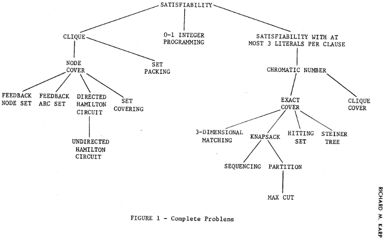
Choosing the starting point could simplify the reduction.
It is an art, with no general recipe.
Summary of NP reductions
An \(\NP\) reduction consists of four parts:
- Description of the reduction \(R\).
- Efficiency of the reduction.
- Completeness: If we are reducing \(A\) to \(B\). If \(x \in A\), then \(R(x) \in B\).
- Soundness: If \(x \not\in A\), then \(R(x) \not\in B\).
P vs NP
“The evidence in favor of [P \(\ne\) NP] and [ its algebraic counterpart ] is so overwhelming, and the consequences of their failure are so grotesque, that their status may perhaps be compared to that of physical laws rather than that of ordinary mathematical conjectures.” — Volker Strassen, laudation for Leslie Valiant, 1986.
“If P=NP, then the world would be a profoundly different place than we usually assume it to be. There would be no special value in “creative leaps,” no fundamental gap between solving a problem and recognizing the solution once it's found. Everyone who could appreciate a symphony would be Mozart; everyone who could follow a step-by-step argument would be Gauss; everyone who could recognize a good investment strategy would be Warren Buffett.” — Scott Aaronson
Course Summary
Chapter 2, 3
Conversion between Automata and Regular Languages (Kleene Construction, State Elimination, Thompson Construction)
Chapter 4
Regular Language Pumping Lemma, Closure Properties of Regular Languages (Closure properties used to prove that a language is not regular), Equivalence and Minimization (will calculate and prove the correctness of the table filling algorithm)
Chapter 5
Context-Free Grammar Design, Simple Proofs Related to Parse Trees, Methods to Eliminate Ambiguity
Chapter 6
Pushdown Automaton Design, Conversion Between Empty Stack and State Acceptance, Bidirectional Conversion with Context-Free Grammar, Characteristics of Deterministic Pushdown Automata
Chapter 7
Grammar Simplification, Grammar Pumping Lemma, Grammar Closure Properties and Related Constructions, Grammar Membership and CYK Algorithm
Chapter 8, 9
Designing Simple Turing Machines, Understanding the Basics of Undecidability, NP Completeness